Evaluating Probability Models

Not sure you’re ready?

Take the ~3-minute readiness diagnostic and see where you stand.

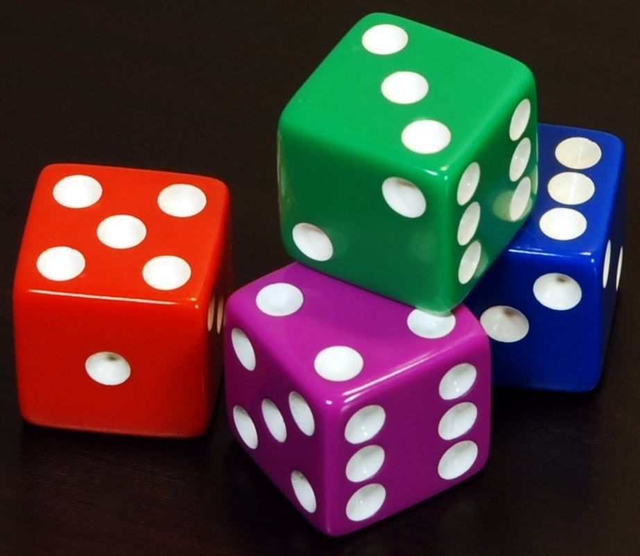
Imagine dropping a standard six-sided die and a standard plastic thumbtack onto a hard classroom floor. Both actions generate unpredictable physical outcomes. Yet, mathematically, we model them entirely differently. We expect the die to land on any of its six faces with equal likelihood because of its perfect symmetry. The thumbtack, however, will land point-up or point-down with starkly different likelihoods dictated by its physical geometry. This distinction forms the bedrock of understanding how we construct mathematical models of chance, how we test those models against the messy reality of experimental data, and how we figure out what went wrong when our mathematical expectations do not match what we see.

A standard six-sided die represents a perfectly uniform probability model due to its physical symmetry.

A thumbtack's asymmetrical physical geometry produces non-uniform outcomes, making it far more likely to land in one specific orientation than the other.

Before we ever flip a coin or spin a spinner in the classroom, we must build a theoretical foundation. Mathematics requires a map before it can navigate the territory.

A probability model is a mathematical representation consisting of a defined sample space and assigned probabilities for each outcome. The sample space is simply the exhaustive set of all possible outcomes for a given probability experiment. If you roll a standard die, the sample space is $\{1, 2, 3, 4, 5, 6\}$ . There are no other possibilities.

A visual representation of a finite sample space detailing an exhaustive set of possible outcomes alongside specifically defined events.

To ensure the model is mathematically valid, it must obey a strict conservation law: the sum of the assigned probabilities for all individual outcomes in a valid probability model must equal exactly one ( $1.0$ , or $100\%$ ).

Uniform vs. Non-Uniform Models

Nature and human design provide us with two distinct types of probability models:

Uniform Probability Model: A uniform probability model assigns the exact same theoretical probability to every individual outcome in the sample space. A fair coin and a fair die are modeled uniformly.
Non-Uniform Probability Model: A non-uniform probability model assigns different theoretical probabilities to at least some individual outcomes in the sample space. The thumbtack from our opening example, or a spinner where the "Red" section takes up half the circle while "Blue" and "Green" take up a quarter each, require a non-uniform model.

How we calculate the likelihood of an event depends entirely on which model we are using:

Calculating Theoretical Probability

In a Uniform Model: The theoretical probability of an event is calculated by dividing the number of favorable outcomes by the total number of possible outcomes. (Example: Rolling an even number on a die is $3$ favorable outcomes out of $6$ total outcomes, or $\frac{1}{2}$ .)

In a Non-Uniform Model: The theoretical probability of an event is calculated by adding the specific assigned probabilities of all outcomes that constitute the event. (Example: On our biased spinner, the probability of landing on "Not Green" is the sum of the probability of Red ( $\frac{1}{2}$ ) and Blue ( $\frac{1}{4}$ ), which equals $\frac{3}{4}$ .)

Theoretical probability is pristine. It describes the mathematically expected outcome without conducting any physical trials. It is what should happen in a perfect universe.

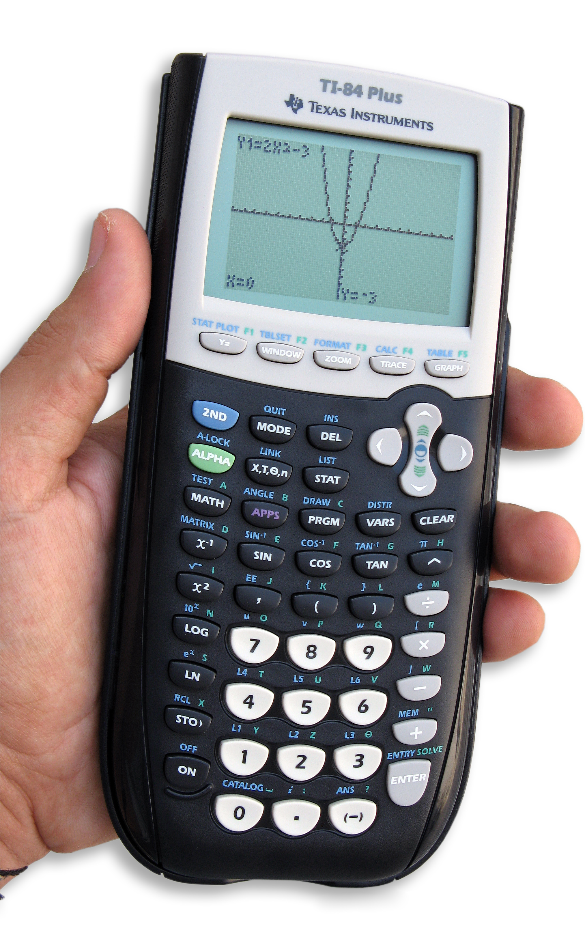
When your middle schoolers actually start flipping coins or running simulations on their graphing calculators, they step out of theory and into reality.

Graphing calculators allow students to bypass manual physical trials, rapidly simulating thousands of expected probabilities to generate robust experimental data.

Experimental probability is the ratio of the number of times a specific event actually occurs to the total number of trials performed. In rigorous statistical contexts, experimental probability is also formally known as empirical probability or relative frequency.

To compare our pristine mathematical map (theory) to the physical territory (experiment), we need a common language. We translate probabilities into frequencies.

Observed frequency is the raw count of how many times a specific outcome happens during an actual experiment. If a student flips a coin $50$ times and sees $28$ heads, the observed frequency is $28$ .
Expected frequency | Expected value is calculated by multiplying the theoretical probability of an event by the total number of experimental trials. For $50$ coin flips, the expected frequency of heads is $\frac{1}{2} \times 50 = 25$ .

Concept	Definition	Example ( $50$ flips of a fair coin)
Theoretical Probability	Mathematically expected outcome.	$P(\text{Heads}) = 0.5$
Expected Frequency	Theoretical probability $\times$ total trials.	$0.5 \times 50 = 25$ expected heads
Observed Frequency	Raw count from an actual experiment.	$28$ heads actually counted
Experimental Probability	Observed frequency / total trials.	$\frac{28}{50} = 0.56$ (Relative Frequency)

Evaluating a probability model involves comparing the generated experimental frequencies against the mathematically expected theoretical frequencies. We are essentially asking: Does the physical reality behave the way our math predicted it would?

When the numbers don't perfectly align, we have a discrepancy. A discrepancy in a probability model refers to a quantitative difference between the expected theoretical frequency and the actual observed frequency. In our coin example, the expected frequency was $25$ , but the observed frequency was $28$ . We have a discrepancy of $3$ .

Is our model broken? Is the coin rigged? Usually, no.

Small discrepancies between expected theoretical frequencies and observed frequencies are entirely normal due to natural sampling variability. Sampling variability is the fundamental statistical principle that observed experimental outcomes will naturally fluctuate randomly across different sets of trials. If every student in your classroom flips a coin $50$ times, almost no one will get exactly $25$ heads, and no two students will get the exact same sequence of flips.

The Great Stabilizer: The Law of Large Numbers

If sampling variability makes every experiment unique, how can we ever trust our theoretical models?

This is where the Law of Large Numbers saves us. This mathematical theorem dictates that as the number of experimental trials increases, the experimental probability will converge toward the theoretical probability.

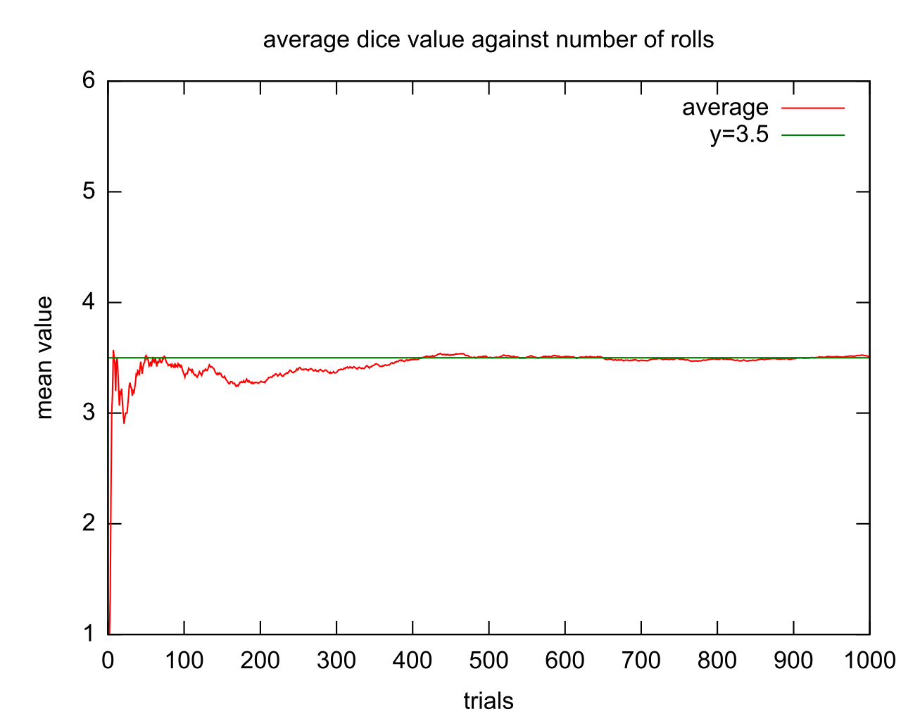
As the number of dice-rolling trials increases, the observed experimental average strictly converges toward the mathematically expected theoretical value, neutralizing sampling variability.

If a student flips a coin $10$ times, getting $8$ heads (an experimental probability of $0.80$ ) is unusual, but not impossible due to sampling variability. But if they use a graphing calculator to simulate $10,000$ flips, the experimental probability will tightly hug the theoretical $0.50$ mark. The "noise" of sampling variability is drowned out by the sheer volume of data.

As a teacher, you will encounter situations where the data absolutely refuses to match the model. When agreement between modeled and observed frequencies is poor, you must help students identify the source of the discrepancy.

Here are the primary culprits you will need to identify on the Praxis 5164 exam and in your classroom:

1. Small Sample Sizes

A small sample size is a primary source of discrepancy between observed frequencies and a mathematically correct theoretical probability model. If a student complains that a die is "broken" because they rolled it four times and never got a $6$ , they are simply victims of a small sample size. The model is fine; the trial count is just too low for the Law of Large Numbers to take effect.

2. Fundamentally Flawed Theoretical Models

If you flip a coin $10,000$ times and observe $7,200$ heads, you no longer have a small sample size. A persistent large discrepancy across a massive number of trials strongly suggests that the underlying theoretical probability model is fundamentally flawed.

This usually happens because we made a false assumption about the physical object. Assuming a physical object like a die or coin is fair when the object is actually weighted leads to an inaccurate uniform probability model. Any inherent physical bias in a randomizing device necessitates the use of a non-uniform probability model to accurately predict long-term expected frequencies.

3. Lack of Statistical Independence

Statistical independence means that the outcome of one trial does not influence the outcome of the next. Experimental trials that lack statistical independence can cause observed frequencies to deviate significantly from the theoretical probability model.

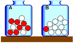
For example, if students are drawing colored marbles from a bag to test a theoretical model but they forget to put the marble back after each draw (drawing without replacement), the probabilities change with every single trial. Their experimental data will heavily disagree with a static theoretical model because the trials are no longer independent.

Drawing colored objects from an urn without replacing them fundamentally alters the probability model for subsequent draws, resulting in events that critically lack statistical independence.

4. Measurement Errors

Sometimes the math is right, and the object is fair, but the humans are flawed. Measurement errors during data collection create artificial discrepancies between observed frequencies and modeled expected frequencies. If a student is dropping a thumbtack but they miscount the tally marks, or they record a "point-up" as a "point-down," the resulting discrepancy is an artifact of bad bookkeeping, not a failure of probability.

Simple observational errors during data collection, such as miscounting handwritten tally marks, create completely artificial discrepancies between mathematical expectations and physical reality.

One of the most profound applications of evaluating probability models in the middle school curriculum is analyzing games.

A fair probability game is mathematically defined as a scenario where all participating players have an equal theoretical probability of winning. If you invent a game where Player A scores a point if a die lands on $1, 2,$ or $3$ , and Player B scores a point if it lands on $4, 5,$ or $6$ , this is a fair game (uniform model, both have a theoretical probability of $\frac{1}{2}$ ).

However, if Player A scores on $1, 2, 3,$ or $4$ and Player B scores on $5$ or $6$ , the game is mathematically unfair. Your students can prove this by creating the non-uniform theoretical model, calculating the expected frequencies, and then running a simulation on their calculators to demonstrate that over the long run (thanks to the Law of Large Numbers), Player A will systematically crush Player B.

By teaching students how to build probability models, how to translate them into expected frequencies, and how to rigorously compare them to observed reality, you are giving them a toolkit to detect bias, understand randomness, and navigate a world governed by chance.