Simple and Compound Probability
Not sure you’re ready?
Take the ~3-minute readiness diagnostic and see where you stand.
When a middle school student flips a coin, rolls a die, or blindly pulls a colored marble from a bag, they are not merely playing a game; they are interacting with the mathematical machinery of uncertainty. Probability is the precise language we use to quantify the unknown. As a mathematics educator, your task is to transform your students' intuitive, often flawed sense of "luck" into a rigorous, algebraic framework. You must teach them to see that chaos has bounds, that randomness has a structure, and that the likelihood of any event can be mapped, calculated, and predicted. Master this architecture, and you equip your students with one of the most powerful analytical tools they will ever encounter in mathematics.
Before we can build complex probabilistic models, we must define the universe in which our experiments take place. This universe is the sample space, defined as the complete set of all possible outcomes of a probability experiment. If you roll a standard six-sided die, the sample space is {1,2,3,4,5,6}.
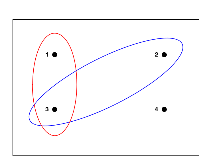
Within this space, we measure the likelihood of specific events.
The Boundaries of Probability The probability of any event is a numerical value ranging from 0 to 1, inclusive.
These boundaries represent the absolute limits of reality. An event with a probability of 0 is an impossible event (e.g., rolling a 7 on a standard six-sided die). At the other extreme, an event with a probability of 1 is a certain event (e.g., rolling a number less than 10).
Because the sample space accounts for everything that could happen, a beautiful conservation law emerges: the sum of the probabilities of all distinct, individual outcomes in a sample space equals exactly 1. The universe of possibilities is entirely accounted for.
Theoretical vs. Experimental Probability
When you ask a student for the probability of rolling a 3, they will quickly tell you it is 61. What they have calculated is the theoretical probability. The theoretical probability of an event is the number of favorable outcomes divided by the total number of equally likely outcomes.
However, reality rarely perfectly matches theory in small doses. If a student actually rolls a die 6 times, they might roll the number 3 twice, or not at all. This lived reality is the experimental probability, which is calculated as the number of times an event occurs divided by the total number of trials performed.
Why do we teach theoretical probability if experiments rarely match it perfectly? Because of a profound mathematical truth known as the Law of Large Numbers.
The Law of Large Numbers states that as the number of trials increases, the experimental probability approaches the theoretical probability.
If your students roll that die 10,000 times instead of 6, the proportion of 3s rolled will inch incredibly close to exactly 61. This is a crucial concept for teaching: it bridges the gap between what we calculate on paper and what happens in the physical world.
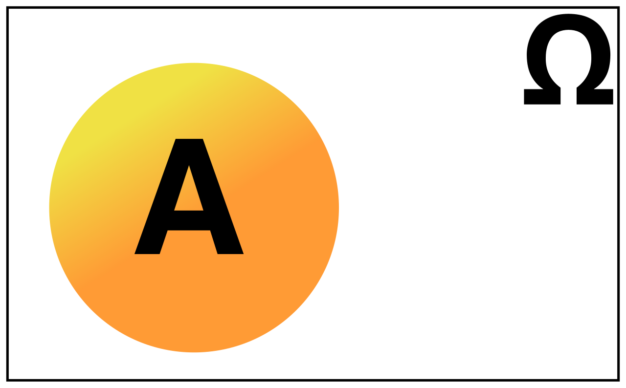
Sometimes, it is mathematically simpler to calculate what won't happen rather than what will.
The complement of an event consists of all outcomes in the sample space that are not in the event. Because the sum of all probabilities in a sample space must equal 1, the probability of the complement of an event equals 1 minus the probability of the event itself:
P(Complement)=1−P(Event)
If the probability of drawing a red marble is 0.3, the probability of drawing a marble that is not red is 1−0.3=0.7.
Mutually Exclusive Events and the Addition Rules
When we begin combining conditions using the word "or," we must ask a critical question: Can these events happen at the same time?
Two events are mutually exclusive if they cannot occur at the same time. For example, a student cannot be simultaneously in the 7th grade and the 8th grade. Because they cannot overlap, the probability of two mutually exclusive events occurring simultaneously is exactly 0.
To find the probability that either of these events happens, we simply combine their individual weights. The probability of either of two mutually exclusive events occurring is the sum of their individual probabilities.
P(A or B)=P(A)+P(B)
But what if the events are not mutually exclusive? What if a student is rolling a die and wants to know the probability of rolling an even number or a prime number? The number 2 is both even and prime. If we simply add P(Even)+P(Prime), we are double-counting the number 2.
To correct for this, we use the general addition rule. The general addition rule states that the probability of either of two events occurring is the sum of their individual probabilities minus the probability of both events occurring.
P(A or B)=P(A)+P(B)−P(A and B)
A compound event is an event that combines two or more simple events. When analyzing compound events—like flipping a coin and then rolling a die—we shift our operational thinking from addition to multiplication.
To determine the total size of our new, expanded sample space, we use the Fundamental Counting Principle. It states that if one event has m possible outcomes and a second event has n possible outcomes, the total number of combined outcomes is m multiplied by n. (e.g., 2 coin outcomes × 6 die outcomes = 12 total combined outcomes).
Independence and Dependence
When events occur in sequence, the most important question an educator must train their students to ask is: Did the first event alter the environment for the second event?
- Two events are independent if the occurrence of one event does not change the probability of the other event occurring. Flipping two distinct coins are independent events; the first coin holds no memory of how it landed, and it exerts no gravitational pull on the second coin.
- Two events are dependent if the occurrence of one event changes the probability of the other event occurring.
The classic pedagogical example involves drawing objects from a container.
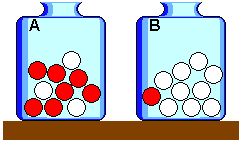
- Drawing items from a set with replacement creates independent events for subsequent draws. The system is reset. The denominator remains the same.
- Drawing items from a set without replacement creates dependent events for subsequent draws. The system is altered. The total number of items has shrunk by one, fundamentally shifting the probabilities for the next draw.
The Multiplication Rules
Calculating the joint probability of events happening in sequence—connected by the word "and"—requires multiplying their probabilities.
For independent events, the math is straightforward. The probability of two independent events both occurring is the product of their individual probabilities:
P(A and B)=P(A)×P(B)
However, if the events are dependent, the probability of the second event is fluid. We must introduce conditional probability, which is the probability of a secondary event occurring given that a primary event has already occurred. We denote this as P(B∣A).
Consequently, the probability of two dependent events both occurring is the probability of the first event multiplied by the conditional probability of the second event:
P(A and B)=P(A)×P(B∣A)
If a bag holds 3 red and 7 blue marbles (10 total), and we draw two marbles without replacement, the probability of drawing Red then Blue is: P(Red)=103 P(Blue∣Red)=97 (Note the denominator shifted because one marble is gone) P(Red and Blue)=103×97=9021
Abstract multiplication rules can alienate middle school learners. To make these concepts tangible, we employ three powerful visual models.
1. Tree Diagrams
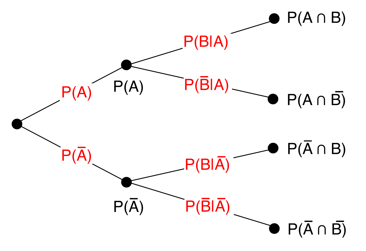
A tree diagram is a graphical representation used to map out the complete sample space of a compound probability experiment. It forces students to explicitly draw out every branching path of reality.
When a student traces a line from the start to the end of a branch, they are tracing a single compound outcome. The probability of a specific outcome path on a tree diagram is calculated by multiplying the probabilities along the branches of that specific path. This visualizes the multiplication rule in a way that feels organic and logical.
2. Area Models
While tree diagrams are excellent for sequential events, geometric models often provide superior intuition for simultaneous, independent events.
An area model uses a grid to represent the probabilities of two independent events by calculating the areas of intersecting sections. Imagine a square with an area of 1. If Event A happens 50% of the time, we shade half the square vertically. If independent Event B happens 20% of the time, we shade one-fifth of the square horizontally. The intersection—the double-shaded rectangle—literally has an area of 0.5×0.2=0.1, proving visually that P(A and B) is 10%.
3. Two-Way Tables
When analyzing real-world data, events are rarely neatly separated into independent dice rolls. We often look at intersections of human traits or choices.
A two-way table displays the frequencies of two categorical variables to help calculate conditional and compound probabilities.
| Prefers Math | Prefers Science | Total | |
|---|---|---|---|
| 7th Graders | 30 | 20 | 50 |
| 8th Graders | 10 | 40 | 50 |
| Total | 40 | 60 | 100 |
Two-way tables are incredibly powerful for teaching conditional probability. If we want to find the probability that a student prefers Math given that they are an 8th grader, the table allows students to visually restrict their sample space. We ignore the entire table except for the "8th Graders" row. Out of those 50 specific students, 10 prefer Math, so the conditional probability is 5010, or 0.2.
By mastering these definitions, boundaries, and visual tools, you transcend simply teaching your students how to plug numbers into fractions. You are giving them the ultimate tool to analyze risk, decode statistics, and make logical, data-driven decisions in a fundamentally uncertain world.