Limits of Functions
Not sure you’re ready?
Take the ~3-minute readiness diagnostic and see where you stand.
Imagine a suspension bridge spanning a deep gorge, structurally flawless except for a single missing wooden plank precisely at its center. If you were to walk from the left side, your path would lead you directly to that exact spatial coordinate. If a friend walked from the right side, their path would point them to that very same coordinate. The bridge is physically broken at that specific point—you cannot step there—but the trajectory of the bridge unequivocally identifies where that step should be.

This is the essence of mathematical limits. The limit of a function describes the value that the function approaches as the input approaches a specific target value. As future mathematics educators, you will find that calculus is built almost entirely upon this framework. When you teach your students the transition from static algebra to dynamic calculus, you are fundamentally teaching them how to interrogate the neighborhood of a point rather than the point itself.
To master the Praxis (5165): Mathematics exam, you must become fluent in the algebraic mechanics, the graphical interpretations, and the rigorous definitions of limits. You must understand not only how to compute them but how to explain why they behave the way they do when a graphing calculator's pixels fail to tell the whole story.
To define a function's behavior rigorously, we must look at how we approach the target.
A left-hand limit evaluates the behavior of a function as the input approaches a specific value strictly from smaller values. Conversely, a right-hand limit evaluates the behavior of a function as the input approaches a specific value strictly from larger values. We denote these with negative and positive superscripts, respectively.
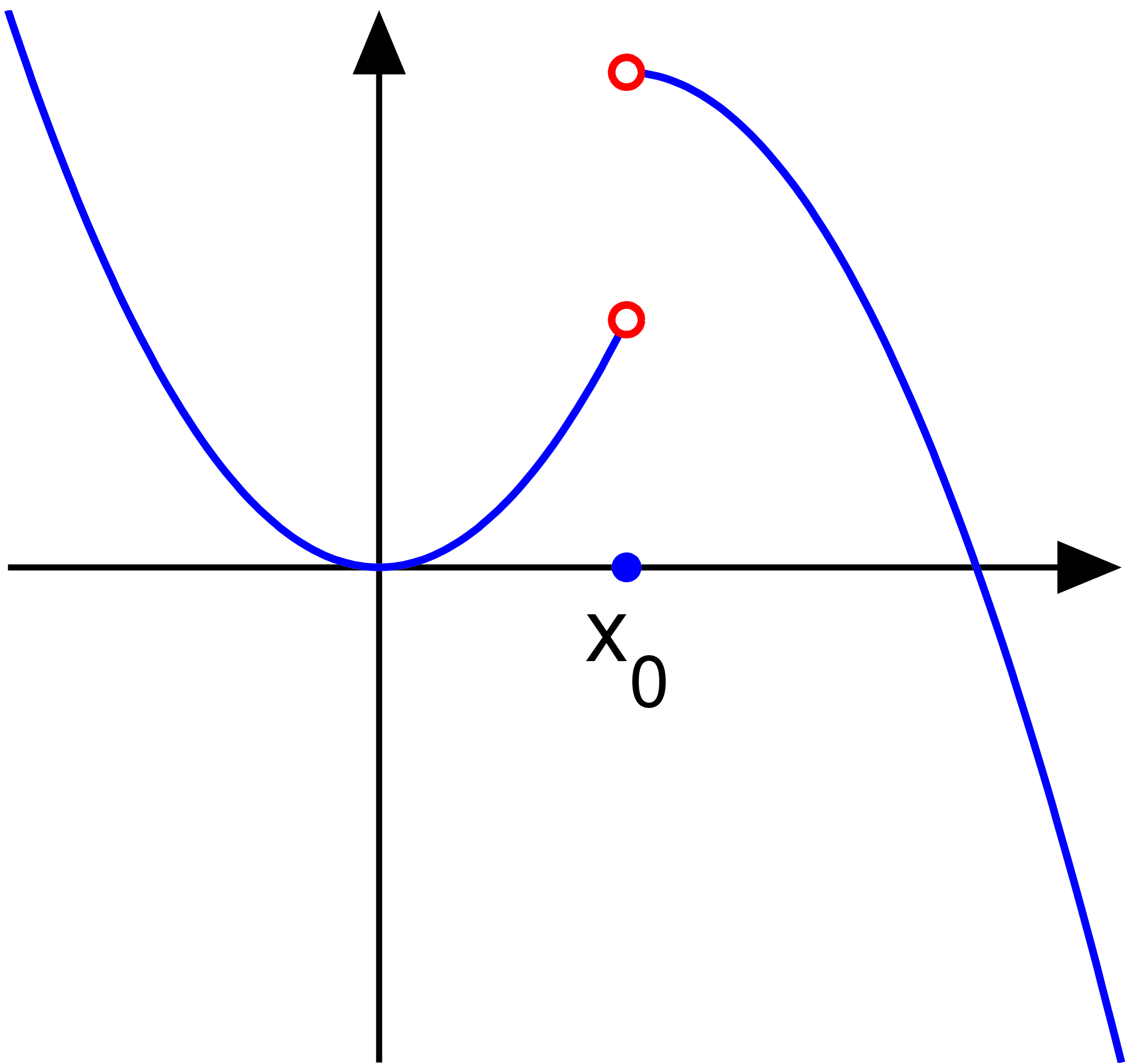
For a function to have a cohesive target, these directional approaches must agree. A two-sided limit requires the corresponding left-hand limit and right-hand limit to evaluate to the exact same real number. If you approach from the left and your friend approaches from the right, and you find yourselves pointing to two entirely different elevations, the overall path is broken. Consequently, a two-sided limit fails to exist if the left-hand limit and the right-hand limit approach different numerical values.
Formalizing the Intuition The formal backbone of this concept is the epsilon-delta definition of a limit. It requires establishing a positive delta (δ) bound on the input for every positive epsilon (ϵ) bound placed on the output. In teaching terms: if a student challenges you to trap the function's output within a microscopic distance (ϵ) of the limit, you can always respond by restricting the input within a tight enough margin (δ) around the target value.

Discontinuities and the Undefined
One of the most critical conceptual leaps for secondary students is realizing that a valid limit can exist at a specific input value even if the function is mathematically undefined at that exact input value.
Consider a rational function with a common factor in the numerator and denominator. Graphically, this manifests as a "hole," or what mathematicians call a removable discontinuity. A limit evaluates perfectly to a finite number at a removable discontinuity. The value of a limit at a removable discontinuity operates independently of the defined function value at that specific coordinate. Whether the function is undefined there, or maliciously redefined to a random point floating above the curve, the limit—the trajectory—remains unchanged.
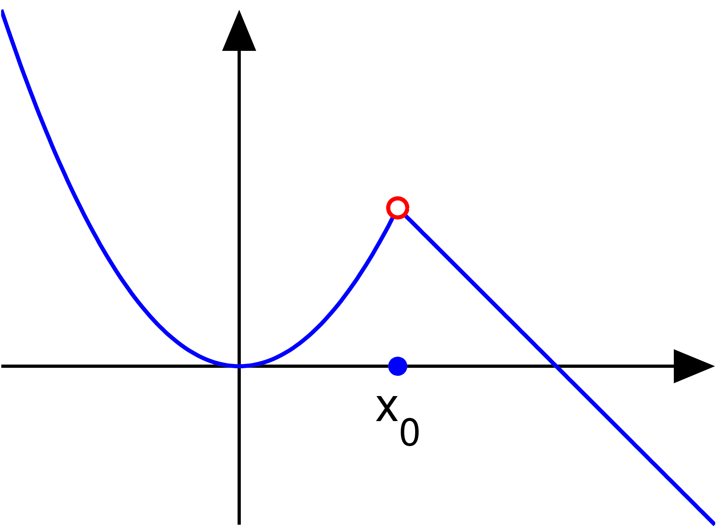
We use this to define continuity itself. A function is classified as continuous at a point if the limit of the function as x approaches the point exactly equals the value of the function at that point. If the limit doesn't match the function value, or if either fails to exist, the function is discontinuous.
When dealing with limits, our primary tool is a set of elegant algebraic rules called Limit Laws. These properties allow us to dismantle complex functions into manageable pieces.
- The Sum Law: The limit of a sum of functions equals the sum of the individual function limits.
- The Difference Law: The limit of a difference of functions equals the difference of the individual function limits.
- The Product Law: The limit of a product of functions equals the product of the individual function limits.
- The Quotient Law: The limit of a quotient of functions equals the quotient of the individual function limits. Crucially, the quotient law for limits is only valid when the limit of the denominator function is not equal to zero.
- The Constant Multiple Law: The limit of a constant multiplied by a function equals the constant multiplied by the limit of the function.
- The Power Law: The limit of a function raised to a specific power equals the limit of the function raised to that same power.
- The Root Law: The limit of the nth root of a function equals the nth root of the limit of the function.
Direct Substitution
Because of these laws, well-behaved continuous functions are a joy to compute. Direct substitution computes the limit of a function at a specific point by evaluating the function exactly at that input value.
Thanks to the predictable nature of algebraic curves, direct substitution successfully evaluates the limit for any polynomial function at any real number. Furthermore, direct substitution successfully evaluates the limit for any rational function at any real number within the domain of the rational function. If the denominator does not vanish, simply plug in the number and compute the result.
What happens when direct substitution yields a zero in the denominator? If the numerator is non-zero (e.g., 5/0), you are looking at a vertical asymptote. But if both evaluate to zero, you have encountered an anomaly.
An indeterminate form zero over zero (0/0) occurs when direct substitution into a limit results in both the numerator and the denominator evaluating to zero. To a novice, 0/0 might look like "undefined" or "one" or "zero." As a teacher, you must emphasize that the indeterminate form zero over zero indicates that further algebraic manipulation is required to evaluate the true value of the limit. It is not an answer; it is a locked door, and algebra is the key.
How do we unlock it?
- Factoring: Often, polynomials hiding a 0/0 form share a hidden root. Factoring can resolve the indeterminate form zero over zero by revealing and canceling common algebraic factors in a numerator and a denominator. Once the offending term (like x−2) is canceled, direct substitution will work perfectly.
- Conjugation: Multiplying by the conjugate expression can resolve the indeterminate form zero over zero in expressions containing square roots. By applying the difference of squares (a−b)(a+b)=a2−b2, we rationalize the numerator or denominator, liberating the hidden algebraic factors so they can be canceled.
L'Hôpital's Rule: The Calculus Escalation
When algebra alone is insufficient or too cumbersome, differential calculus steps in. L'Hôpital's Rule evaluates the limit of an indeterminate form zero over zero by computing the limit of the quotient of the derivatives. It is equally powerful for infinite behaviors: L'Hôpital's Rule evaluates the limit of an indeterminate form infinity over infinity by computing the limit of the quotient of the derivatives.
However, beware of a common student pitfall. The application of L'Hôpital's Rule strictly requires the limit of the quotient of the derivatives to evaluate to a real number or infinity. You cannot apply it if the resulting limit oscillates wildly or if the initial form was not indeterminate.
Sometimes, algebraic manipulation and derivatives fail, particularly with trigonometric functions. In these moments, we rely on containment.
The Squeeze Theorem (or Sandwich Theorem) guarantees that a function squeezed between two other converging functions will share the common limit of the outer functions at that specific point. If Function A is always less than or equal to Function B, and Function B is always less than or equal to Function C, and both A and C approach a limit of L at a certain point, then B has no choice but to be squeezed to L as well.
This elegant logic gives us two foundational facts necessary for evaluating complex trigonometric limits on your exam:
Limits do not just govern tiny, localized points; they are the language we use to describe the grand, infinite boundaries of functions.
Vertical Asymptotes: The Infinite Limit
An infinite limit occurs when the output values of a function grow without bound as the input approaches a specific finite value. If you plug in a value closer and closer to x=3, and the outputs balloon to 100, 10,000, and 1,000,000, the limit is infinity. Geometrically, an infinite limit at a specific finite x-value graphically indicates the presence of a vertical asymptote at that x-value.
Horizontal Asymptotes: Limits to Infinity
Conversely, what happens to a function as time marches on indefinitely? A limit to infinity evaluates the end behavior of a function as the input variable increases or decreases without bound. If this settling process converges, a finite limit to infinity graphically indicates the presence of a horizontal asymptote.
For rational functions, the end behavior is delightfully predictable. The limit of a rational function at infinity depends entirely on the ratio of the term with the highest degree in the numerator to the term with the highest degree in the denominator. Lower-degree terms become mathematically negligible as x approaches infinity.
Here is the taxonomy of rational function limits at infinity, a must-know for secondary curriculum:
| Degree Comparison | Limit Evaluation as x→±∞ | Graphical Meaning |
|---|---|---|
| Numerator < Denominator | A rational function whose numerator degree is strictly less than its denominator degree has a limit of zero at positive and negative infinity. | Horizontal Asymptote at y=0 (the x-axis). |
| Numerator = Denominator | A rational function whose numerator degree equals its denominator degree has a limit at infinity equal to the ratio of the leading coefficients. | Horizontal Asymptote at y=ba. |
| Numerator > Denominator | A rational function whose numerator degree is strictly greater than its denominator degree evaluates to positive or negative infinity as the input approaches infinity. | No Horizontal Asymptote (possible slant asymptote). |
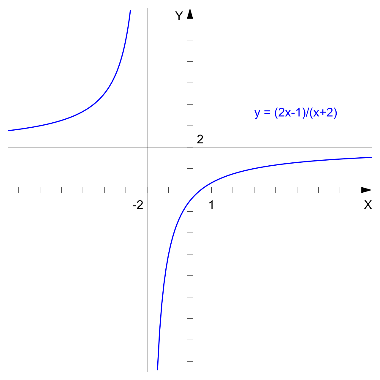
The Engine Behind End Behavior Why do these degree rules work? Because the limit of a constant divided by x to the power of n, as x approaches infinity, evaluates to zero for any positive rational number n. (limx→∞xnC=0). When you divide every term in a rational function by the highest power of x, all lower-degree terms vaporize to zero, leaving only the leading ratio.
The Birth of a Constant
While infinity is often used to describe rational polynomials, it also gives birth to exponential wonders. The mathematical constant e equals the limit of the quantity one plus one over x, all raised to the power of x, as x approaches infinity. e=limx→∞(1+x1)x This specific limit to infinity is the heartbeat of continuous compounding interest and exponential decay, concepts your future students will encounter frequently.
We have discussed limits that converge smoothly and limits that shoot to infinity. But limits can also shatter entirely. A limit fails to exist in a few distinct, pathological scenarios that often appear as conceptual questions on the Praxis exam.
- The Jump Discontinuity: Commonly seen in piecewise functions or absolute value quotients (like x∣x∣), a jump discontinuity prevents a two-sided limit from existing due to the left-hand and right-hand limits approaching different finite values. The path literally teleports from one elevation to another.
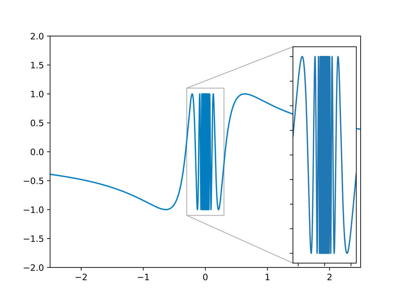
- Infinite Oscillation: A limit fails to exist if a function oscillates infinitely between multiple different values as the input approaches a specific target point. The classic, textbook example of this phenomenon is the function defined by the sine of one over x. This function (sin(1/x)) exhibits infinite oscillation and has no valid limit as x approaches zero. If you zoom in on a graphing calculator at x=0, the screen fills with a solid block of ink because the wave bounces between −1 and 1 infinitely fast. It never settles, and therefore, it cannot be said to approach any single, numerical target.
When you stand in front of a whiteboard to teach these concepts, remember that limits are the ultimate tool for asking, "What is happening exactly here, without looking exactly here?"
You must be able to deploy the Limit Laws efficiently, recognize when direct substitution gives you a clear answer, and interpret an indeterminate form (0/0 or ∞/∞) not as an error, but as a command to factor, conjugate, or apply L'Hôpital's Rule. You must visualize how finite limits to infinity dictate horizontal asymptotes, and how infinite limits at finite points reveal vertical asymptotes. And most importantly, you must be able to explain the nuanced distinction between a function's defined value and its limit at a removable discontinuity.
Master these principles, and you will not only conquer the limits questions on your exam, but you will also possess the clarity required to guide your future students across the bridge into higher mathematics.