Modeling Periodic Phenomena

Not sure you’re ready?

Take the ~3-minute readiness diagnostic and see where you stand.

A pendulum swinging in a grandfather clock, the rhythmic rise and fall of coastal tides, and the seasonal progression of daylight hours all share a profound mathematical architecture. They are governed by periodic phenomena—systems that repeat their behavior over predictable, endless intervals. To model these systems mathematically is to capture the heartbeat of the physical world. In the secondary mathematics classroom, transitioning students from static algebraic lines to the dynamic, oscillating curves of trigonometric functions is a pivotal conceptual leap. This requires more than memorizing equations; it demands a deep structural understanding of how geometric parameters stretch, shift, and constrain sinusoidal waves to perfectly mirror reality.

The dynamic curve of a sine wave unrolling from the periodic circular motion of a unit circle perfectly illustrates the continuous, repeating nature of periodic phenomena.

To map a physical reality to a mathematical model, we rely on the standard form of a sinusoidal function. We write these models as either $y = a \sin(b(x - h)) + k$ or $y = a \cos(b(x - h)) + k$ . Every parameter in these equations has a direct physical interpretation.

Midline and Amplitude: The Vertical Dimensions

A wave must oscillate around a center of equilibrium. The parameter $k$ represents this vertical shift, explicitly defining the midline $y = k$ , which is the horizontal line halfway between the maximum and minimum values of the periodic function.

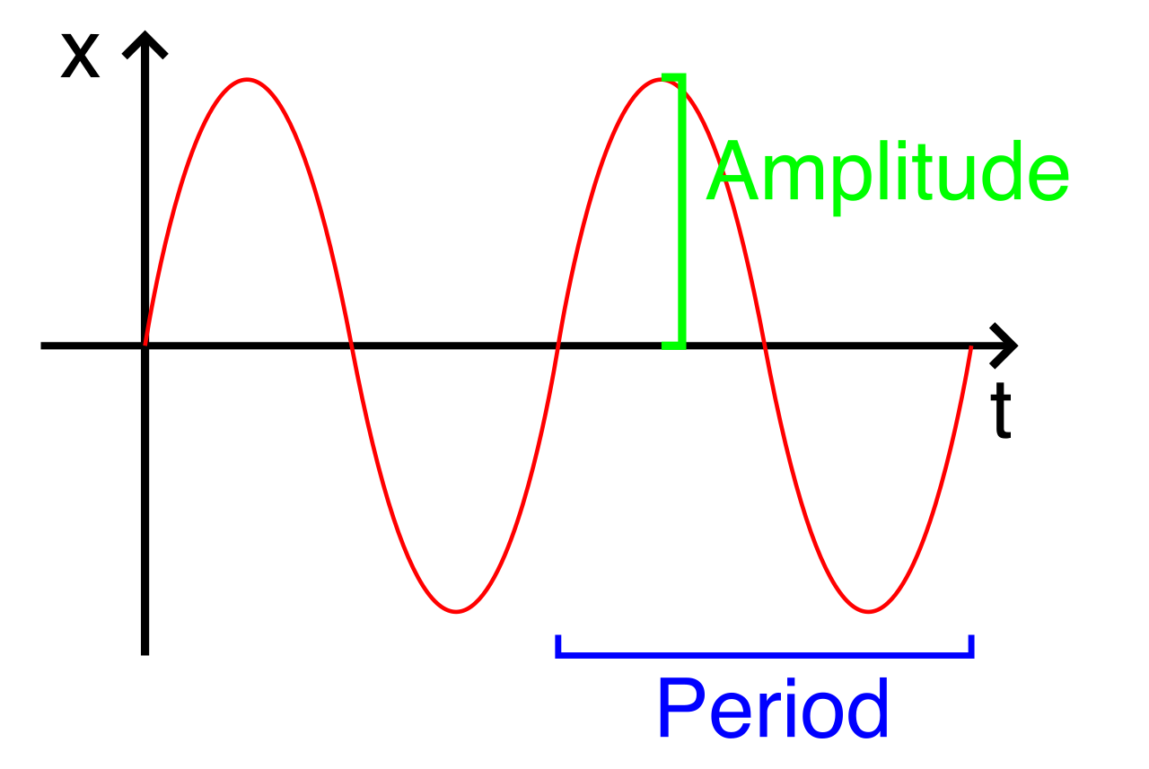
The energy or intensity of the wave is given by its amplitude. By definition, the amplitude is half the difference between the maximum and minimum values of a periodic function. In our standard forms, the parameter $|a|$ represents the amplitude.

When you establish $k$ and $|a|$ , you instantly define the strict vertical boundaries of your model:

The maximum value of the sinusoidal model is exactly $k + |a|$ .
The minimum value of the sinusoidal model is exactly $k - |a|$ .

Period and Frequency: The Horizontal Dimensions

If the vertical dimensions tell us how far a wave travels, the horizontal dimensions tell us how often it repeats. The period is the length of one complete cycle of a periodic function. It is governed by the parameter $b$ using the formula:

$\text{Period} = \frac{2\pi}{|b|}$

Closely related to the period is frequency, which is the reciprocal of the period. While the period measures the length of the independent variable (often time) required to complete one cycle, the frequency represents the number of complete cycles a periodic function undergoes per unit of the independent variable. For instance, if a wheel completes a rotation every $\frac{1}{4}$ of a second (period), its frequency is $4$ rotations per second.

A graphical representation of a wave showing the period as the horizontal length of one complete cycle between consecutive peaks.

Phase Shift: Aligning the Clock

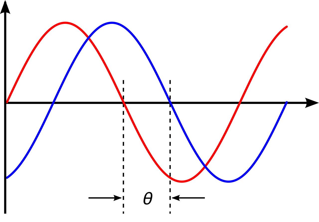
Finally, the parameter $h$ represents the phase shift, which is the horizontal displacement of a periodic function from the standard position of the parent trigonometric function. This parameter is simply the mathematical equivalent of setting the hands on a clock; it aligns the mathematical wave with the specific starting time $x = 0$ of our observed phenomenon.

A phase shift translates a periodic wave horizontally, allowing the mathematical model to align accurately with the initial timing of an observed phenomenon.

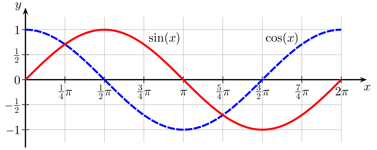
One of the most common instructional hurdles is teaching students to decide between using a sine function or a cosine function when building a model. Because sine and cosine are simply horizontal translations of one another, either can be used. However, choosing the correct parent function based on initial conditions dramatically simplifies the phase shift $h$ .

Cosine functions model phenomena starting at a maximum or minimum value when the phase shift is zero. If you are modeling a weight pulled down on a spring and released at time $t = 0$ , you start at a minimum. Cosine is the natural choice, allowing $h = 0$ (and $a < 0$ ).
Sine functions model phenomena starting at the midline when the phase shift is zero. If you are modeling a pendulum pushed from its resting equilibrium position at time $t = 0$ , sine is the elegant choice, preserving $h = 0$ .

The sine and cosine parent functions are identical in shape but offset by a horizontal phase shift, allowing modelers to choose the most convenient function based on initial conditions.

Classic Real-World Contexts

When building these models, real-world modeling constraints dictate the relevant domains and parameters. You must familiarize your students with standard natural cycles:

Annual Temperatures: When modeling annual temperature variations over a year, the period is typically set to $12$ months or $365$ days. Setting $\frac{2\pi}{|b|} = 12$ immediately gives $b = \frac{\pi}{6}$ .
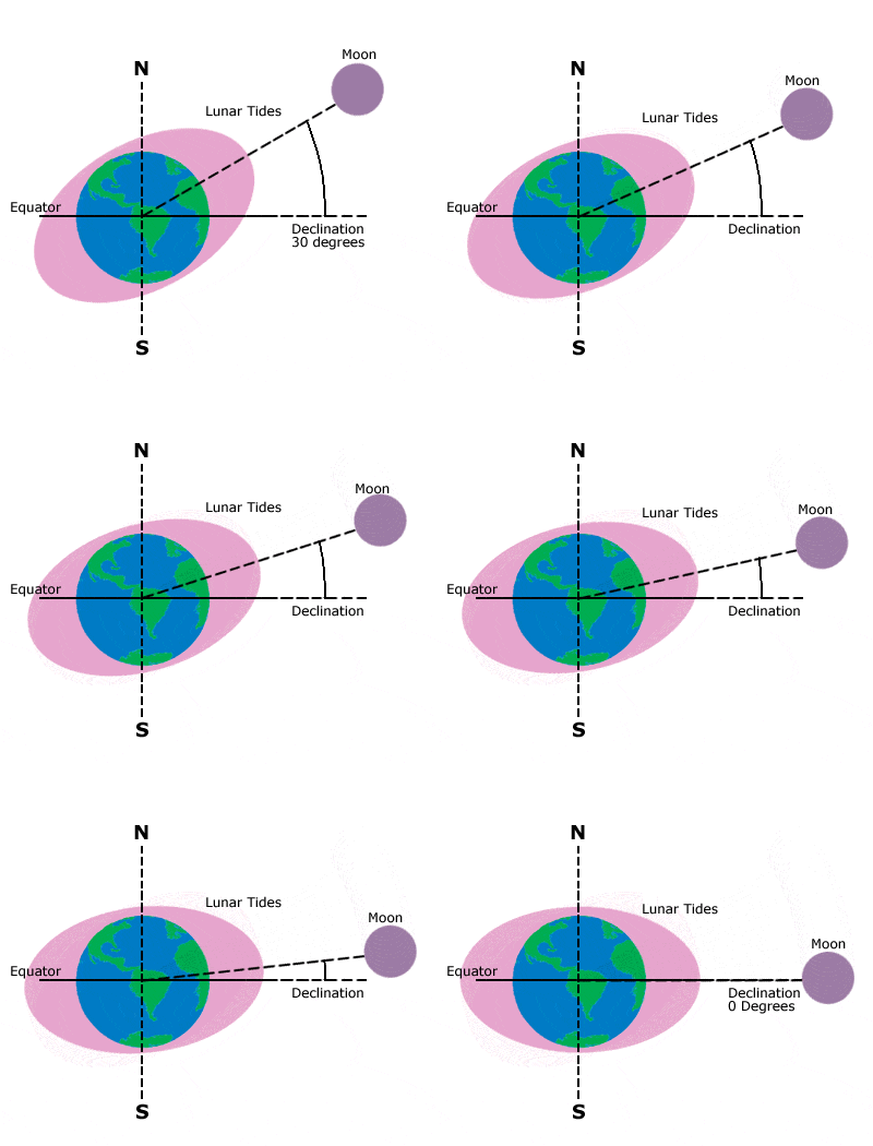
Ocean Tides: Due to the gravitational interplay between the Earth, Moon, and Sun, tidal changes do not happen exactly every 12 hours. When modeling tidal changes over a single day, the period is approximately $12.4$ hours.

A simplified animation of Earth's tides demonstrating how lunar gravitational pull creates periodic, predictable changes in sea level over consistent time intervals.

To use these models to make predictions—such as finding when the tide will be high enough for a ship to enter a harbor—we must solve equations. This necessitates working backward from a known output to an unknown input, leading us to inverse trigonometric functions.

There is an immediate mathematical crisis here: sine, cosine, and tangent fail the horizontal line test infinitely many times. Therefore, inverse trigonometric functions require restricted domains of the parent trigonometric functions to satisfy the definition of a true mathematical function (which dictates that one input yields exactly one output).

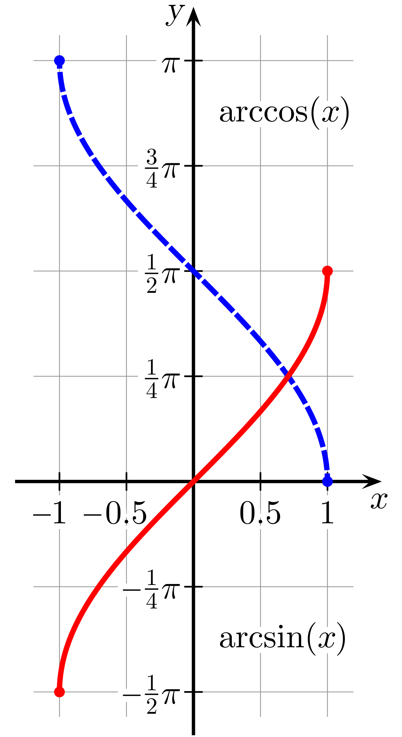
Inverse trigonometric functions output an angle measure corresponding to a given trigonometric ratio. We must memorize the strict domain restrictions placed on the parent functions, which in turn define the ranges of the inverse functions:

Function	Restricted Domain of Parent	Range of Inverse Function	Meaning of the Inverse
Sine	$[-\pi/2, \pi/2]$	$[-\pi/2, \pi/2]$	$\arcsin(x)$ represents the angle $\theta$ in $[-\pi/2, \pi/2]$ such that $\sin(\theta) = x$ .
Cosine	$[0, \pi]$	$[0, \pi]$	The restricted domain of $y = \cos(x)$ used to create $\arccos(x)$ is $[0, \pi]$ .
Tangent	$(-\pi/2, \pi/2)$	$(-\pi/2, \pi/2)$	The restricted domain of $y = \tan(x)$ used to create $\arctan(x)$ is $(-\pi/2, \pi/2)$ .

When an inverse trigonometric function is evaluated, it yields the principal value—the single, specific solution to a trigonometric equation obtained directly from the inverse function within these defined boundaries.

The restricted domains of the arcsine (red) and arccosine (blue) functions are strictly defined to ensure each input yields exactly one principal value output.

When solving the equation $a \sin(b(x - h)) + k = c$ , the algebraic process is systematic.

Step 1: Isolate the Trigonometric Expression

Before applying an inverse function, you must strip away the amplitude and midline. Solving the equation involves isolating the trigonometric expression to find:

$\sin(b(x - h)) = \frac{c - k}{a}$

Step 2: Find the Principal and Secondary Solutions

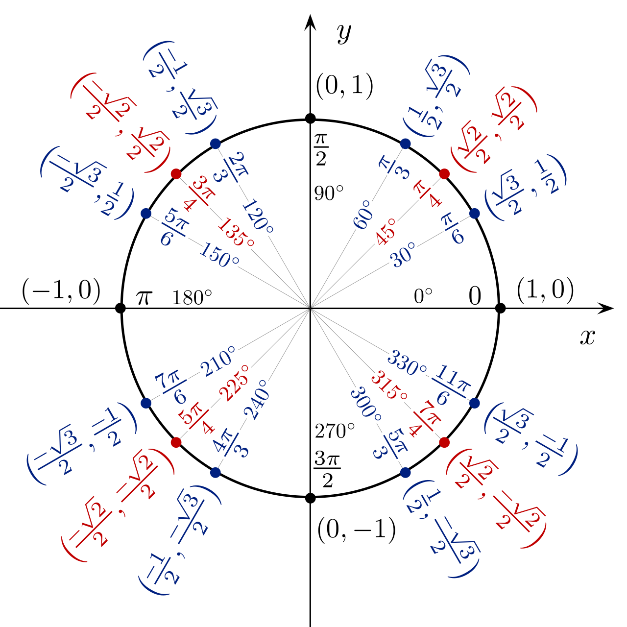
Applying the inverse sine function (e.g., $\arcsin$ ) to $\frac{c - k}{a}$ yields the principal value. However, the physical phenomenon occurs more than once per cycle. We must find the secondary solutions within one period. We rely on the profound geometric symmetries of the unit circle:

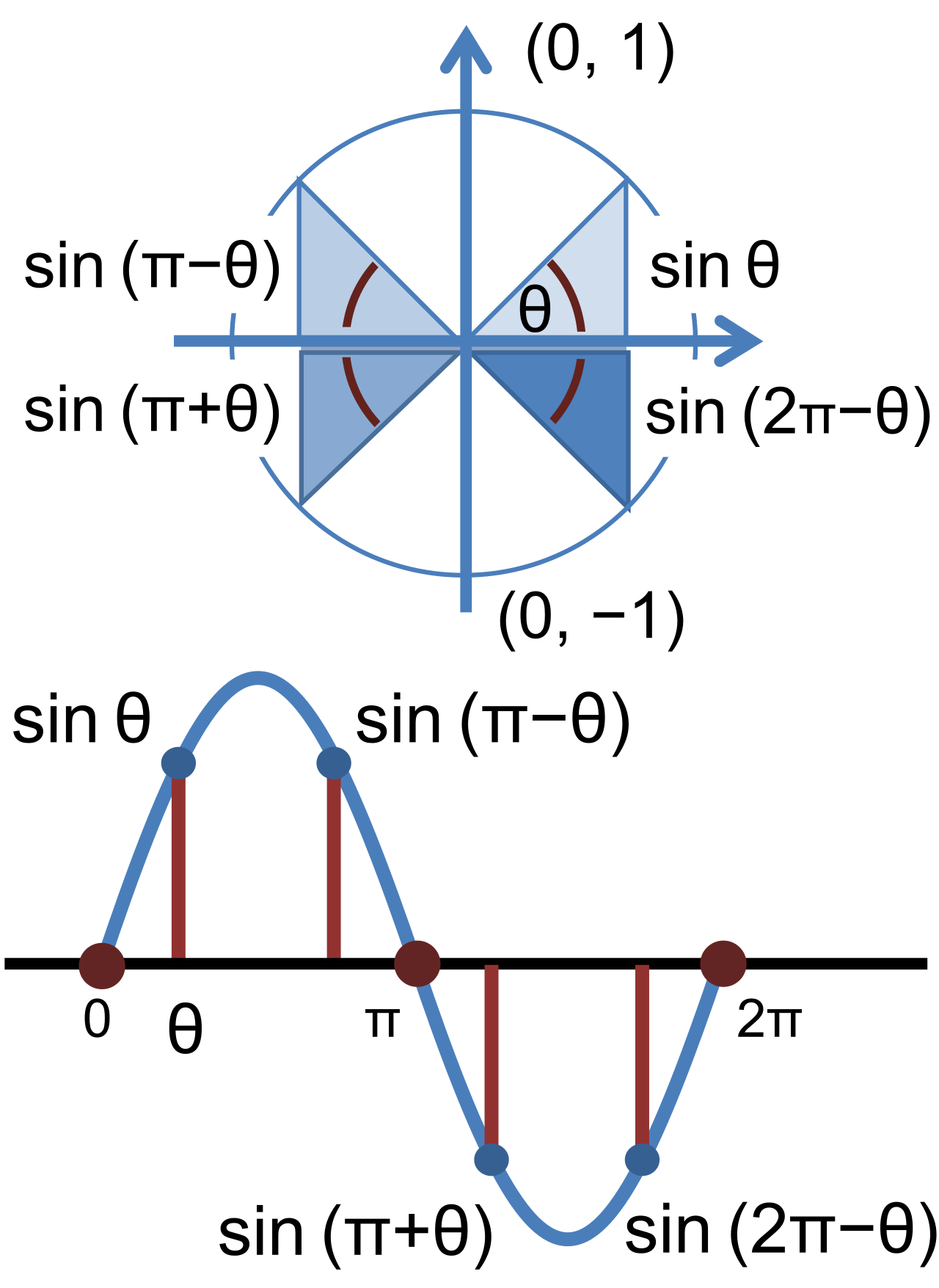
Secondary solutions within one period of a sine function are found using the symmetry property $\sin(\theta) = \sin(\pi - \theta)$ . If the sea level hits 10 feet on the way up, it will hit 10 feet again on the way down.
Secondary solutions within one period of a cosine function are found using the symmetry property $\cos(\theta) = \cos(2\pi - \theta)$ .

The symmetries of the unit circle are essential for finding all secondary solutions to trigonometric equations within a single period.

Step 3: Expand to Infinity, Then Constrain to Reality

Trigonometric equations often have infinitely many solutions due to the periodic nature of trigonometric functions. Adding integer multiples of the period to base solutions yields the complete infinite set of solutions for a trigonometric equation. If your period is 12 months, you add $12n$ (where $n$ is an integer) to your base solutions.

Finally, we apply our context. Real-world modeling constraints dictate the relevant domain of solutions for trigonometric equations. If we are only concerned with tidal changes over a single 24-hour day, we filter our infinite set of solutions, keeping only those where $0 \le t \le 24$ .

As an educator, you must recognize that modeling periodic phenomena relies heavily on technological proficiency. A graphing calculator is a vital tool, but it will only yield correct answers if the machine's parameters match the mathematical context.

Crucially, a graphing calculator must be set to the correct angle mode to evaluate trigonometric and inverse trigonometric functions accurately for a given context. In almost all continuous algebraic modeling scenarios—like temperature, sound waves, or tides—calculators must be set to Radian mode. Degrees are an arbitrary human construct of 360 units; radians represent the pure relationship between radius and arc length, allowing input variables (like hours or days) to scale correctly against real numbers.

A graphing calculator dynamically plotting a sine wave. When modeling continuous real-world phenomena, calculators must be properly configured to Radian mode to correctly scale inputs against real numbers.

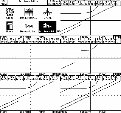
Furthermore, when algebraic isolation is too complex, students can utilize the intersection method on a graphing calculator. This method finds solutions to $f(x) = g(x)$ by determining the intersection points of the graphs of $y = f(x)$ and $y = g(x)$ . For example, to find when the tide $f(x)$ reaches $8$ feet, one simply graphs the tidal model $y_1 = f(x)$ alongside the horizontal line $y_2 = 8$ and uses the calculator's intersect command to locate the precise coordinates where the mathematical model perfectly intersects the physical requirement.