The Derivative

Not sure you’re ready?

Take the ~3-minute readiness diagnostic and see where you stand.

If you photograph a speeding car, the image freezes the vehicle in a single instant of time. Yet, we intuitively understand that the car possesses velocity—a rate of change—even within that frozen, durationless instant. Resolving the paradox of how an object can be changing at a moment when time itself is paused is the defining triumph of differential calculus. The derivative provides the exact mathematical machinery to capture this instantaneous behavior. As educators, guiding students from the tangible reality of average speeds over measurable distances to the abstract concept of instantaneous change at a single point requires bridging the finite and the infinitesimal.

To understand instantaneous change, we must first look at average change. Geometrically, average change is represented by a secant line, which is a line that intersects a function's graph at two distinct points.

When you compute the slope of this secant line, you are determining the average rate of change of the function over the specific interval between those two points. The algebraic expression used to find the slope of a secant line is called the difference quotient.

But average change over an interval is not our end goal; we seek the change at a specific moment. Imagine sliding the second point of intersection along the curve closer and closer to the first point. As the distance between the two points shrinks, the sequence of secant slopes begins to stabilize, approaching a single, definitive value.

The slope of the tangent line is the limit of the slopes of the secant lines as the distance between the two points approaches zero.

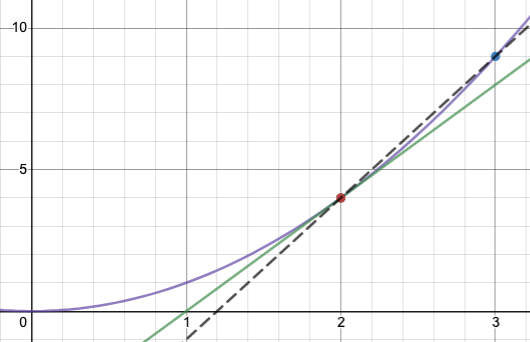
As the two points defining a secant line move closer together, the secant line's slope converges to that of the tangent line, visually representing the limit that defines instantaneous change.

A tangent line represents the best linear approximation to a curve at a specific point. If you were to zoom in infinitely close to that point on the graph, the curve and its tangent line would become indistinguishable. Consequently, the slope of a tangent line represents the instantaneous rate of change of a function at a single point. For the simplest functions—like a linear function $f(x) = mx + b$ —the rate of change never varies; thus, its derivative is constantly equal to the slope $m$ .

In the 17th century, Isaac Newton and Gottfried Wilhelm Leibniz independently developed the foundational concepts of calculus to formalize these ideas. To express the derivative algebraically, we rely on the limit of the difference quotient.

The Formal Limit Definition of the Derivative: For a function $f(x)$ , the derivative $f'(x)$ is defined as: $f'(x) = \lim_{h \to 0} \frac{f(x+h) - f(x)}{h}$

There is also an alternative limit definition tailored for finding the derivative at a specific point $a$ : $f'(a) = \lim_{x \to a} \frac{f(x) - f(a)}{x - a}$

Notice the evolution of notation here. The prime notation $f'(x)$ for the derivative was introduced by Joseph-Louis Lagrange. However, it was Gottfried Wilhelm Leibniz who introduced the fractional notation $\frac{dy}{dx}$ . The related notation $\frac{d}{dx}$ acts as an operator, indicating the mathematical operation of taking the derivative with respect to the variable $x$ .

A manuscript by Gottfried Wilhelm Leibniz, who introduced the foundational fractional notation for derivatives and integrals still used today.

When you teach students to evaluate the limit definition algebraically, you must equip them with distinct algebraic toolkits depending on the function family they are analyzing. Substitution of $h = 0$ initially yields the indeterminate form $\frac{0}{0}$ , requiring algebraic manipulation:

Polynomial functions: Evaluating the limit definition often requires expanding binomials (using the Binomial Theorem or Pascal's Triangle) and factoring out the variable $h$ from the numerator to cancel with the denominator.
Rational functions: These limits typically require finding a common denominator to combine fractions in the numerator before simplifying.
Radical functions: Evaluating these limits frequently requires multiplying the numerator and denominator by a conjugate expression to eliminate the radical from the numerator, a process called rationalizing the numerator.

The formal difference quotient is asymmetrical—it steps forward by a distance $h$ . However, a more balanced approach exists, known as the symmetric difference quotient, defined as the expression: $\frac{f(x+h) - f(x-h)}{2h}$

The limit of the symmetric difference quotient as $h$ approaches zero provides the exact derivative of the function. This is not merely an academic exercise; it is the hidden mechanism inside modern technology. Graphing calculators often approximate the numerical derivative at a point using the symmetric difference quotient for a very small value of $h$ (typically $h = 0.001$ ).

You will frequently encounter exam items that ask you to estimate a derivative from a data table. Evaluating a derivative from a data table requires calculating the average rate of change between adjacent data points. Just like the graphing calculator, using left and right points around a target value in a data table provides a more accurate derivative approximation than using a single-sided interval.

A central theme in secondary mathematics is understanding where mathematical rules break down. We must clearly define the relationship between continuity and differentiability.

Continuity is a necessary condition for a function to have a derivative at a point. Therefore, a function must be continuous at a specific point to be differentiable at that specific point.

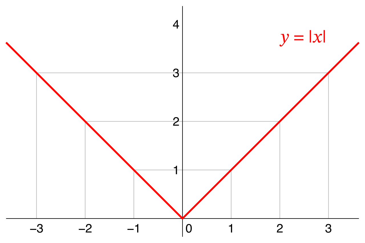
However, continuity is not a sufficient condition to guarantee that a function is differentiable at a point. The classic counterexample you must keep in your instructional arsenal is the absolute value function, $f(x) = |x|$ .

The absolute value function $f(x) = |x|$ is continuous at $x = 0$ .
The absolute value function $f(x) = |x|$ is not differentiable at $x = 0$ .

Why does it fail? Because as you approach $x = 0$ from the left, the slope of the secant lines is always $-1$ . As you approach from the right, the slope is $+1$ . The limit of the slopes does not exist because the left-hand and right-hand limits disagree.

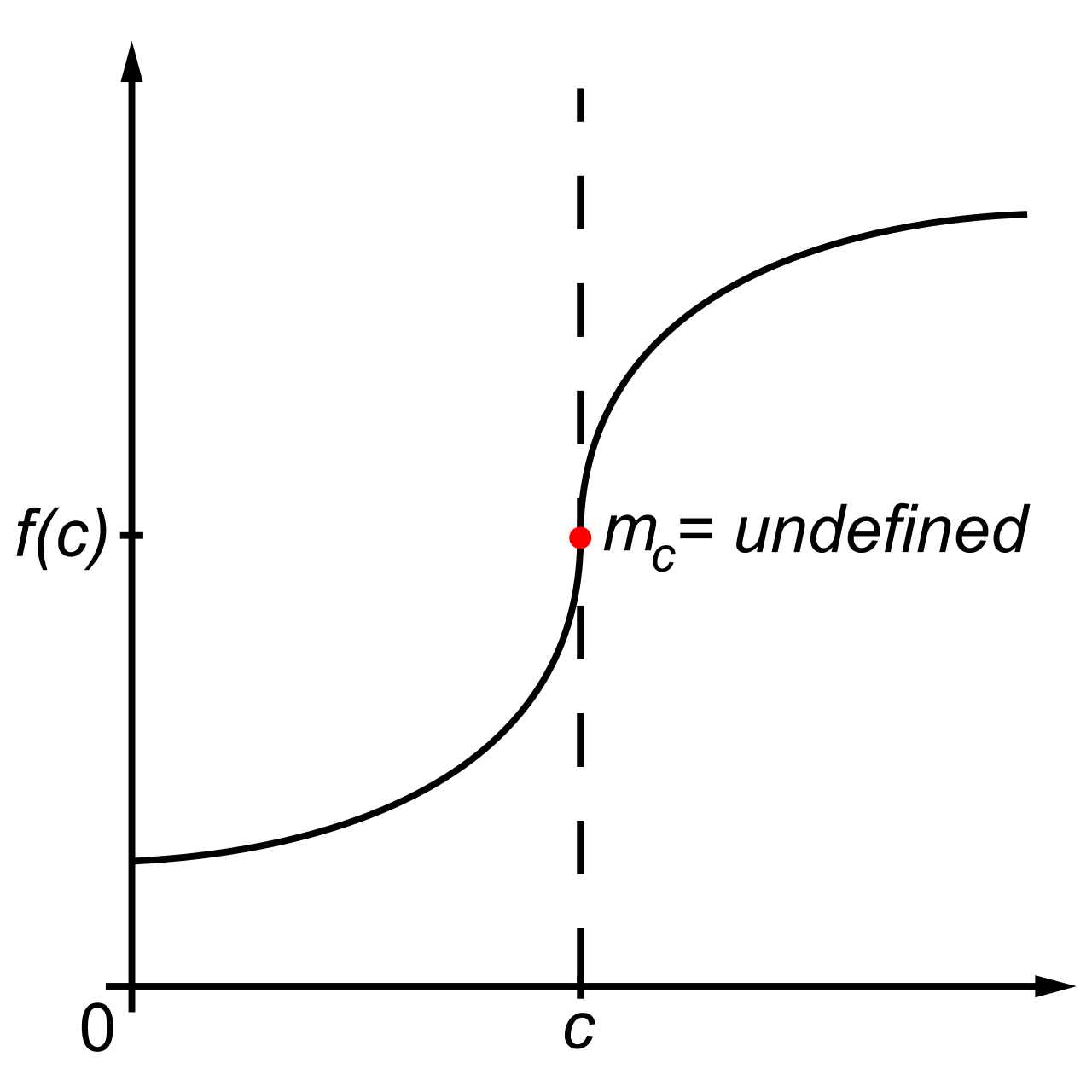
The absolute value function is continuous at the origin but fails to be differentiable there due to its sharp corner, which causes the left-hand and right-hand limits of the slopes to disagree.

Visually, we can classify the points where a function fails to be differentiable:

A function fails to be differentiable at any point where the graph exhibits a sharp corner (like $f(x) = |x|$ ).
A function fails to be differentiable at any point where the graph exhibits a cusp (like $f(x) = x^{2/3}$ at $x=0$ ).
A function fails to be differentiable at any point where the graph possesses a vertical tangent line (like $f(x) = \sqrt[3]{x}$ at $x=0$ , where the difference quotient limit approaches infinity).

At a vertical tangent, the difference quotient limit approaches infinity, leaving the derivative undefined despite the function remaining continuous.

To truly master the derivative, a teacher must be able to translate it across various real-world contexts. The power of calculus is that the same mathematical operation models vastly different physical realities.

Units and Behavior

No matter the context, the units of a derivative $\frac{dy}{dx}$ are always the units of the dependent variable $y$ divided by the units of the independent variable $x$ .

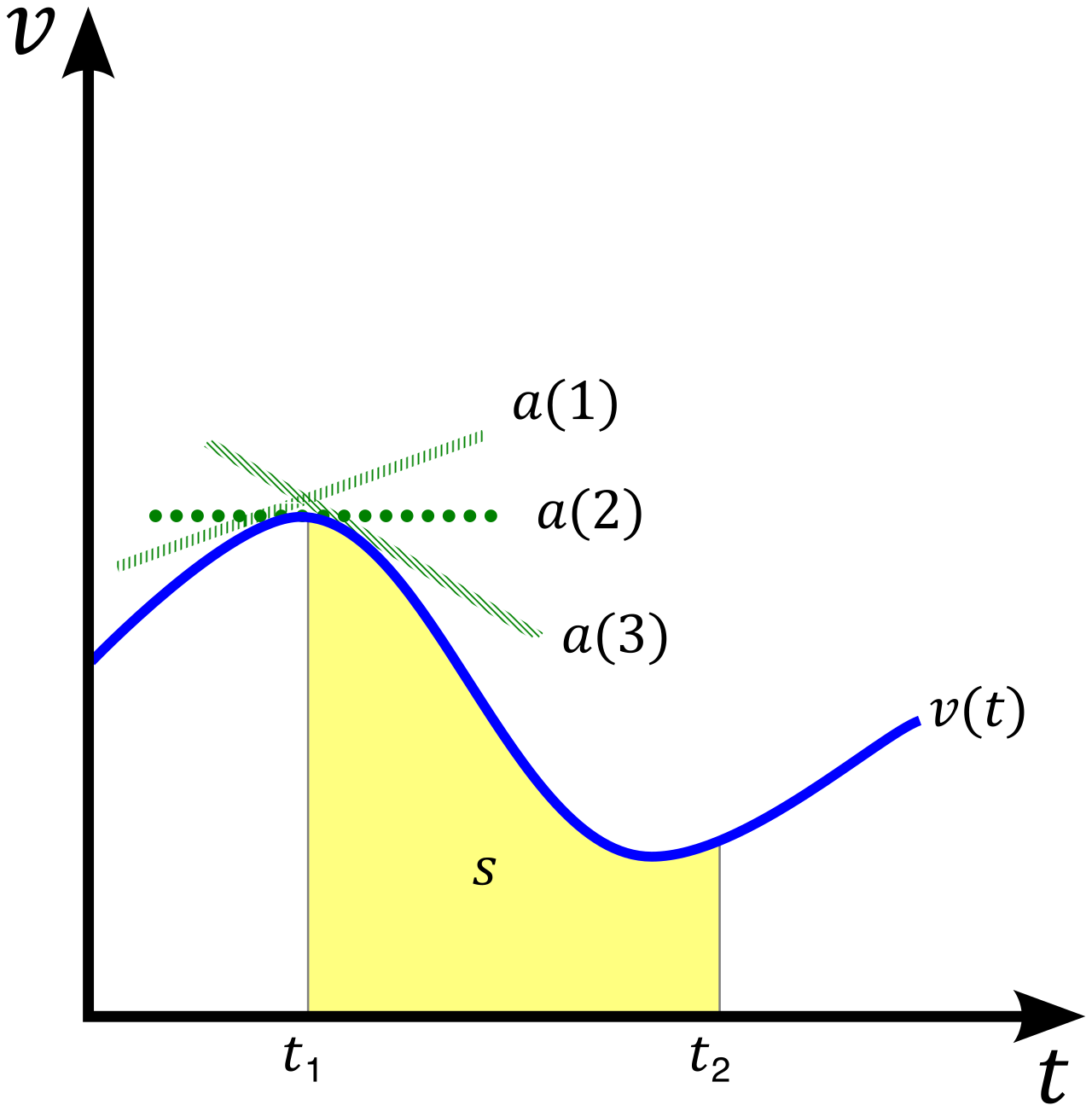
The sign of the derivative tells us the behavior of the original function. A strictly positive derivative over an interval indicates that the original function is strictly increasing on that interval. Conversely, a strictly negative derivative over an interval indicates that the original function is strictly decreasing on that interval. When a continuous curve smoothly transitions from increasing to decreasing (or vice versa), the tangent line becomes perfectly horizontal. Therefore, the derivative evaluated at a local maximum or local minimum of a differentiable function equals zero.

Kinematics

In physics, we track objects moving through space.

The derivative of a position function with respect to time yields the instantaneous velocity function. (Units: meters per second).
The derivative of a velocity function with respect to time yields the instantaneous acceleration function. (Units: meters per second squared).
Instantaneous speed is defined mathematically as the absolute value of the instantaneous velocity function. Velocity has direction (indicated by its sign); speed is a strictly non-negative magnitude.

In kinematics, acceleration can be determined by evaluating the derivative—represented by the slopes of tangent lines—at any given point along a velocity versus time curve.

Economics

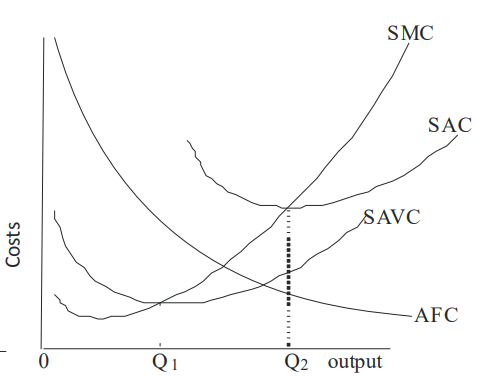
In business and economics, the derivative measures the cost or benefit of producing "one more unit."

The derivative of a total cost function with respect to the number of items produced is called the marginal cost. If it costs $\$ 5,000$ to produce 100 units, the marginal cost tells us the approximate cost to produce the 101st unit.
The derivative of a total revenue function with respect to the number of items sold is called the marginal revenue.

In economic models, the marginal cost curve (MC) represents the derivative of the total cost function, indicating the approximate cost to produce one additional unit.

When you stand before a classroom, your task is to unify multiple representations of the derivative. Your students need to see that the geometric slope of the tangent line, the algebraic limit of the difference quotient, the numerical approximation on their graphing calculators, and the physical reality of a car's speedometer are all describing the exact same concept. By grounding the abstract limits in concrete, contextual rates of change—from marginal cost to instantaneous acceleration—you give students the conceptual anchors they need to thrive in advanced mathematics.