Standard Differentiation Techniques

Not sure you’re ready?

Take the ~3-minute readiness diagnostic and see where you stand.

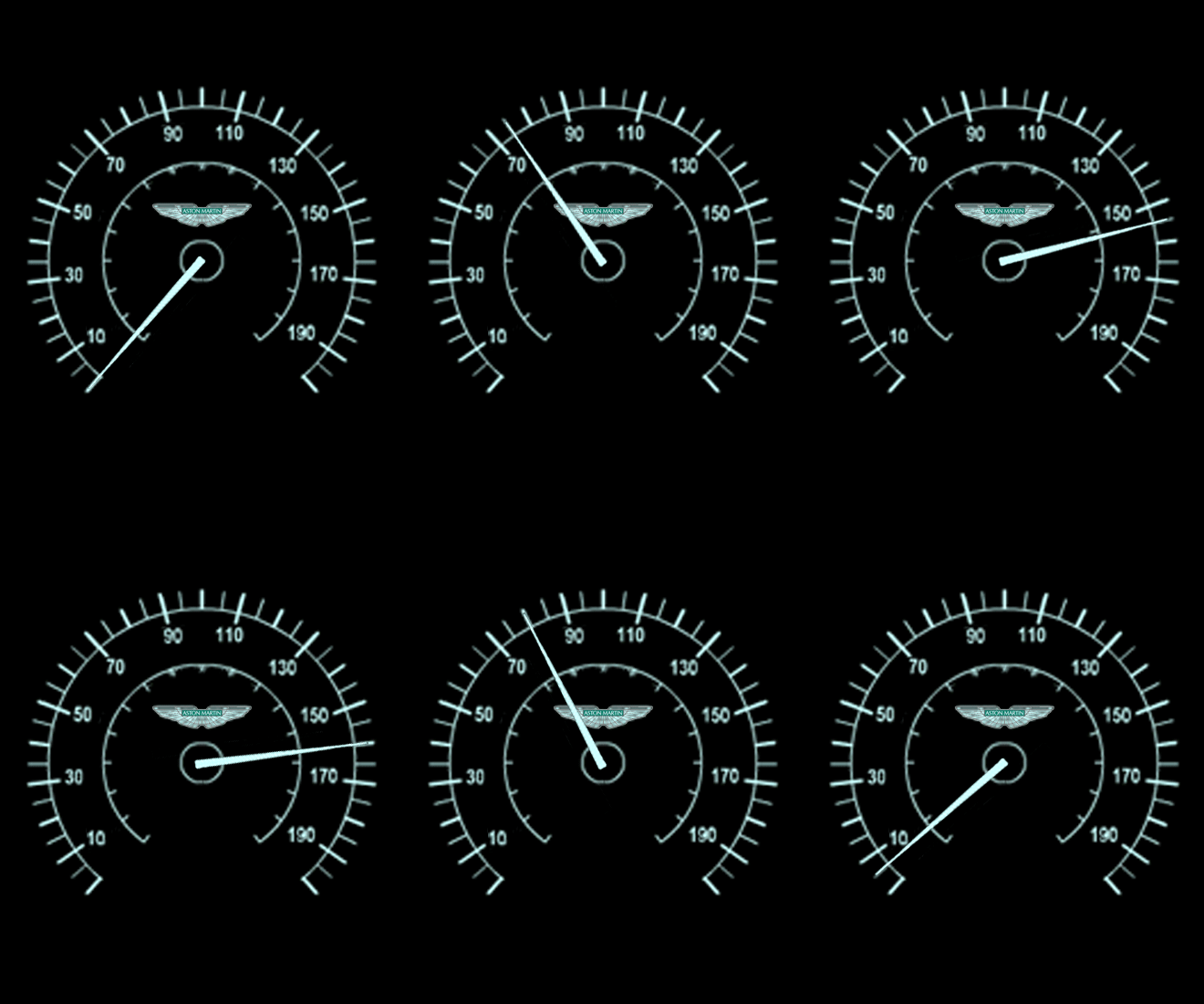
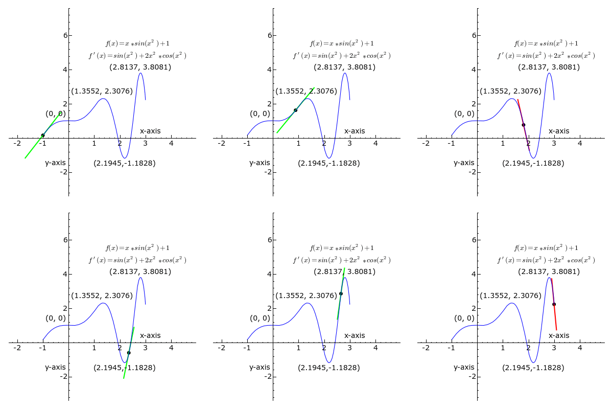
Imagine a vehicle moving down a highway, its position continuously tracked over time. Algebra can tell us exactly where the vehicle is at any given second, or calculate its average speed over an hour. But algebra fails if we want to read the speedometer at a frozen instant. To capture that exact, momentary reality, we rely on the derivative. Fundamentally, the derivative of a function represents the instantaneous rate of change of the function with respect to the input variable. Geometrically, the derivative of a function at a specific point represents the slope of the tangent line to the graph of the function at that exact point.

An analogue speedometer captures the instantaneous rate of change of a vehicle's position, illustrating the real-world meaning of the derivative.

Geometrically, the derivative evaluated at a specific point is the slope of the line tangent to the function's curve at that coordinate.

As a future secondary mathematics educator, your goal on the Praxis (5165): Mathematics exam—and in your classroom—is not merely to memorize operations, but to master the architecture of these rates of change. When students plug functions into a graphing calculator, the machine blindly connects pixels. Your job is to understand and explain the invisible boundaries, domains, and rules that govern these mathematical behaviors.

Graphing calculators display functions by filling discrete pixels, which can hide the continuous nature or sudden undefined boundaries of mathematical domains.

Before calculating a derivative, we must ensure the derivative actually exists. The relationship between continuity and differentiability is a frequent trap on selected-response exams.

The core logical absolute is this: Differentiability of a function at a specific point logically implies continuity of the function at that same point. If a curve is smooth enough to have a defined tangent line, it cannot have a break, hole, or jump.

However, the converse is strictly false. Continuity of a function at a specific point does not guarantee differentiability of the function at that point. A continuous road can suddenly jag. Visually and mathematically, a function fails to be differentiable at three specific graphical features:

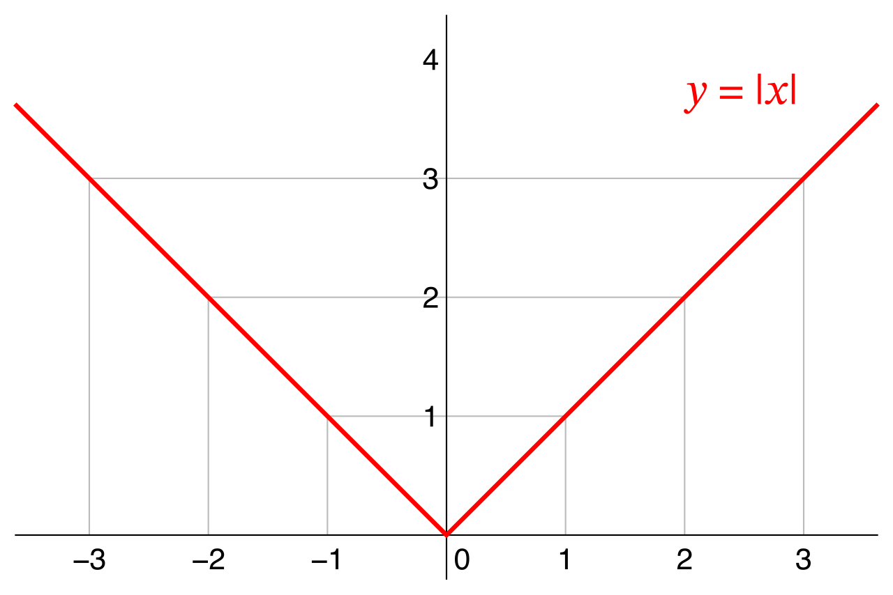
Sharp corners: Such as the vertex of the absolute value function, $f(x) = |x|$ at $x=0$ , where the slope instantly snaps from $-1$ to $1$ .

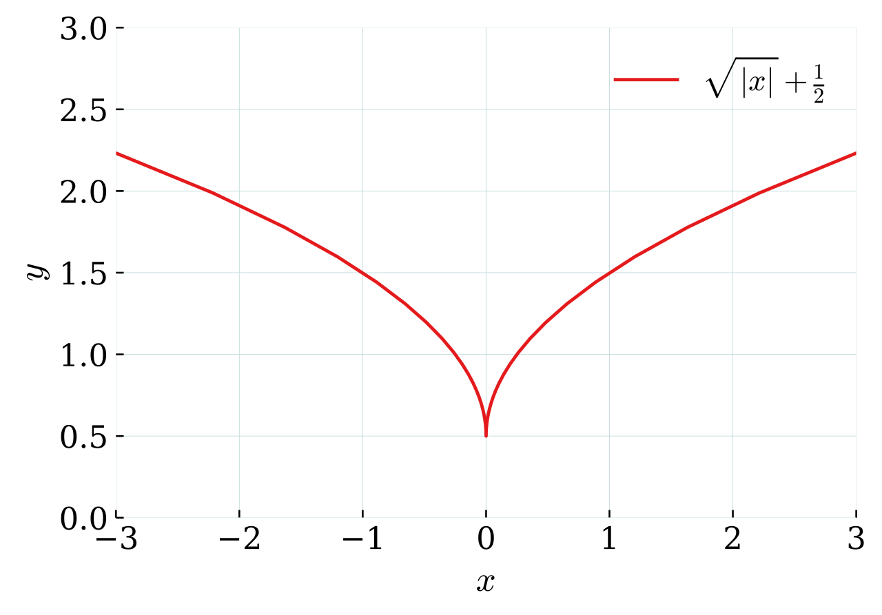
The absolute value function possesses a sharp corner at its vertex, making it continuous but not differentiable at that specific point.

Cusp points: Such as $f(x) = x^{2/3}$ at $x=0$ , where the curve pinches inward, sending the slope toward infinity from one side and negative infinity from the other.

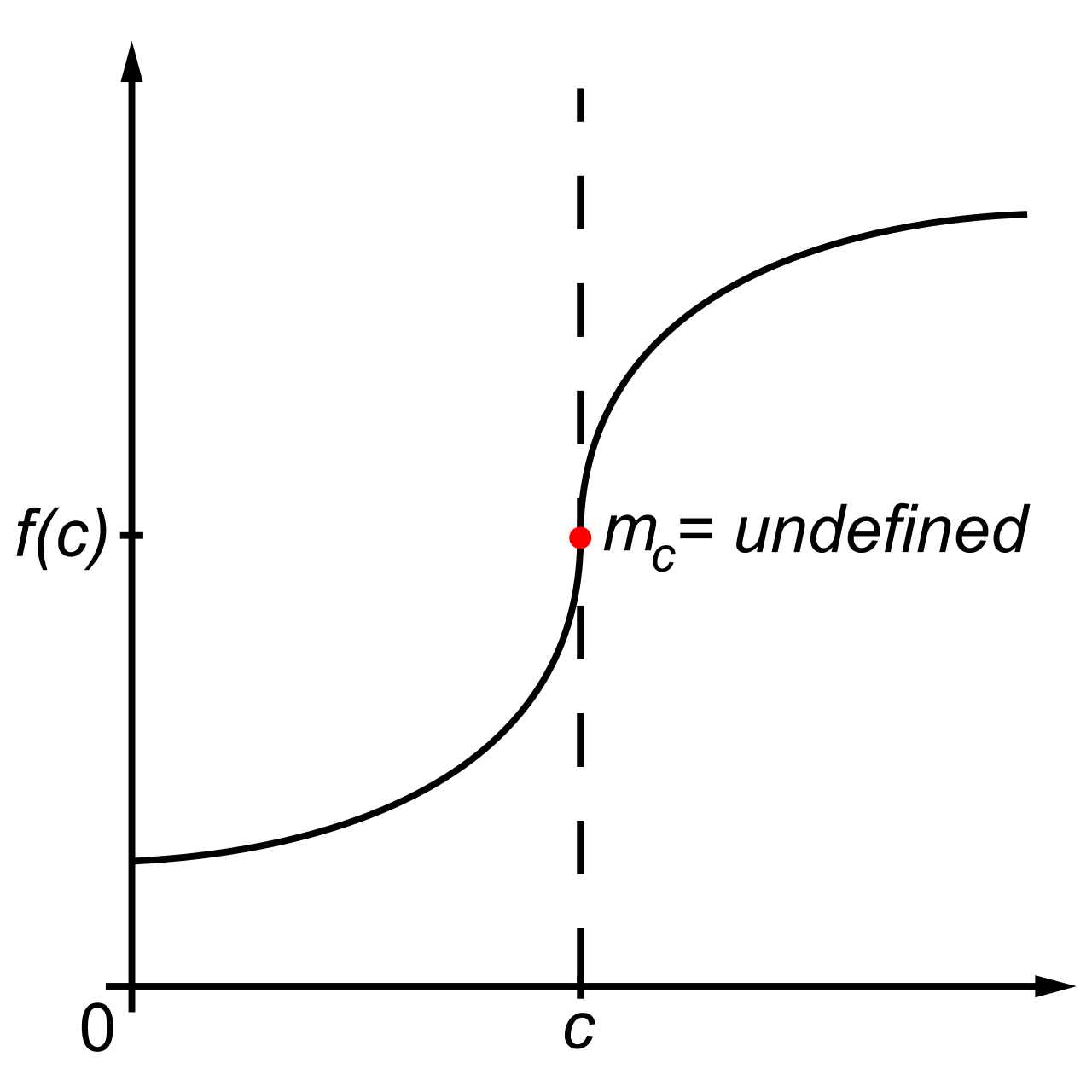
A cusp occurs when a curve pinches inward, driving the tangent slope toward infinity and causing differentiability to fail.

Vertical tangent lines: Such as $f(x) = x^{1/3}$ at $x=0$ , where the curve goes momentarily, perfectly vertical, resulting in an undefined slope.

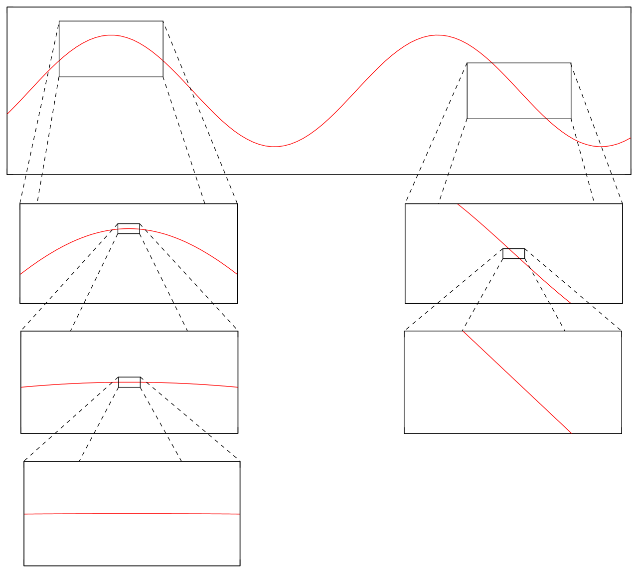
When a curve possesses a vertical tangent, its slope becomes momentarily undefined, meaning the derivative does not exist at that point.

When teaching, encourage students to zoom in on their graphing calculators. If they zoom in infinitely on a differentiable point, the curve will eventually look exactly like a straight line (local linearity). If they zoom in on a corner or cusp, it will stubbornly remain jagged.

If a function is differentiable, zooming in sufficiently on a point will reveal local linearity, where the curve appears indistinguishable from its tangent line.

Once we know a function is differentiable, we systematically deconstruct it using foundational rules.

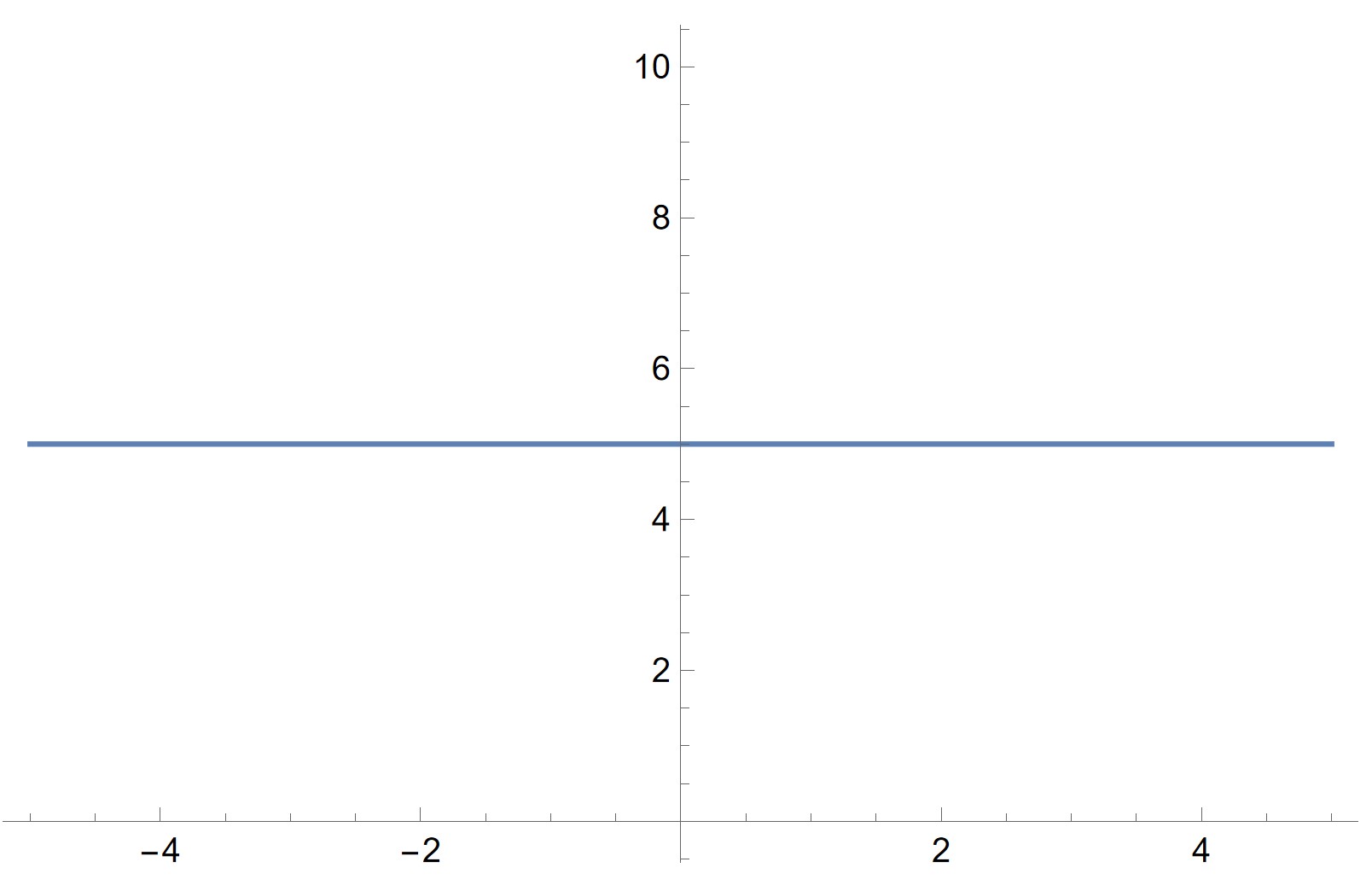
The Constant Rule: The derivative of a constant function is zero. If a value never changes, its rate of change is zero. Geometrically, $f(x) = 5$ is a horizontal line; its slope everywhere is zero.

The graph of a constant function is a perfectly horizontal line; because its value never changes, its slope and derivative are exactly zero everywhere.

The Power Rule: The power rule states the derivative of $x$ to the power of $n$ is $n$ times $x$ to the power of $n$ minus one: $\frac{d}{dx}[x^n] = n x^{n-1}$ . Crucially, the power rule for differentiation applies to any real number exponent. It works just as flawlessly for $f(x) = x^{\pi}$ as it does for $f(x) = x^2$ .

When functions are scaled, added, or subtracted, calculus respects the linear nature of these operations:

Constant Multiple Rule: The constant multiple rule states the derivative of a constant multiplied by a function is the constant multiplied by the derivative of the function. $\frac{d}{dx}[c \cdot f(x)] = c \cdot f'(x)$ .
Sum Rule: The sum rule states the derivative of a sum of functions is the sum of the individual derivatives of the original functions. $\frac{d}{dx}[f(x) + g(x)] = f'(x) + g'(x)$ .
Difference Rule: The difference rule states the derivative of a difference of functions is the difference of the individual derivatives of the original functions.

Linearity stops when functions are multiplied or divided. The rate of change of a rectangle's area depends not just on how fast its length and width are growing, but on how long and wide the rectangle currently is.

The Product Rule

The product rule states the derivative of $f(x)$ multiplied by $g(x)$ is the derivative of $f(x)$ multiplied by $g(x)$ plus $f(x)$ multiplied by the derivative of $g(x)$ . $\frac{d}{dx}[f(x)g(x)] = f'(x)g(x) + f(x)g'(x)$

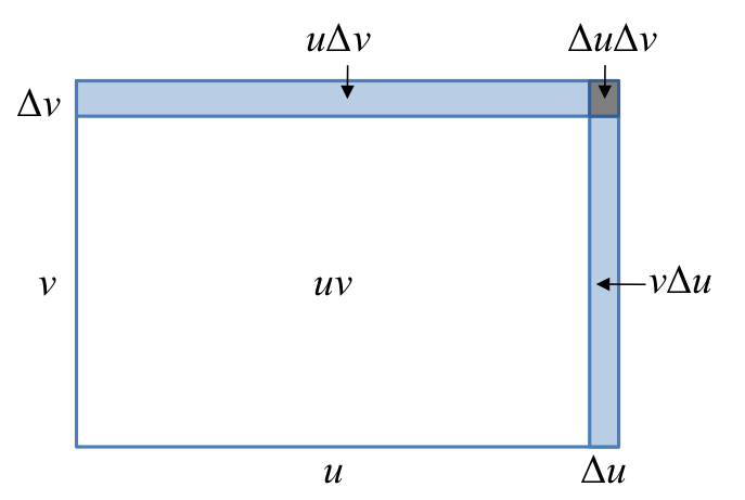
When encountering more complex models, evaluating the derivative of a product of three or more functions requires iterative application of the product rule. For instance, to differentiate $f(x)g(x)h(x)$ , you treat $[f(x)g(x)]$ as a single function, apply the rule, and then apply the rule again within the resulting expansion.

The Quotient Rule and Reciprocals

The quotient rule states the derivative of $f(x)$ divided by $g(x)$ is the derivative of $f(x)$ multiplied by $g(x)$ minus $f(x)$ multiplied by the derivative of $g(x)$ , all divided by the square of $g(x)$ . $\frac{d}{dx}\left[\frac{f(x)}{g(x)}\right] = \frac{f'(x)g(x) - f(x)g'(x)}{[g(x)]^2}$

A vital domain constraint applies here: The quotient rule requires the denominator function to be non-zero at the point of evaluation. If $g(x) = 0$ , the function is undefined, and the derivative is consequently undefined.

Often, students face a constant divided by a function, such as $\frac{1}{x^3 + 2}$ . Instead of the full quotient rule, we use a more efficient shortcut. The reciprocal rule is a special case of the quotient rule used to differentiate the constant one divided by a function $g(x)$ . By setting $f(x) = 1$ (and thus $f'(x) = 0$ ) in the quotient rule, we find that the derivative of the constant one divided by a function $g(x)$ is the negative derivative of $g(x)$ divided by the square of $g(x)$ . $\frac{d}{dx}\left[\frac{1}{g(x)}\right] = \frac{-g'(x)}{[g(x)]^2}$

In the real world, functions are nested. The heat of a metal plate depends on the distance from a fire, and the distance from the fire depends on time. To find how heat changes with time, we must link these rates together. The chain rule is used to differentiate composite functions.

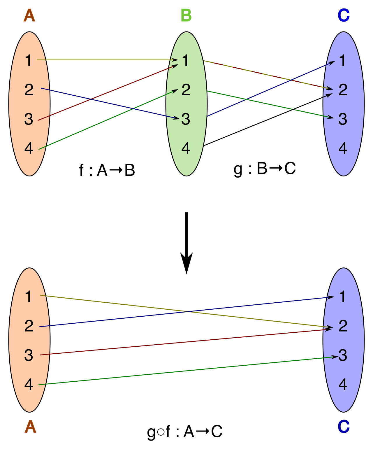
The chain rule governs the differentiation of composite functions, where the output of an inner function serves directly as the input for an outer function.

The chain rule states the derivative of $f(g(x))$ is the derivative of the outer function $f$ evaluated at the inner function $g(x)$ , multiplied by the derivative of the inner function $g(x)$ . $\frac{d}{dx}[f(g(x))] = f'(g(x)) \cdot g'(x)$

This is beautifully and mathematically expressed using Leibniz notation as $dy/dx$ equals $dy/du$ multiplied by $du/dx$ . This fractional notation is highly intuitive for secondary students; they can visualize the $du$ terms "canceling out" (even though they are operators, not true fractions) to reveal the final rate of change.

Furthermore, the chain rule can be applied recursively to differentiate functions composed of three or more nested functions. If we have $f(g(h(x)))$ , we peel it like an onion from the outside in: differentiate $f$ keeping $g(h(x))$ intact, multiply by the derivative of $g$ keeping $h(x)$ intact, and finally multiply by the derivative of $h(x)$ .

Transcendental functions (exponentials and logarithms) model natural phenomena, from compound interest to radioactive decay.

Exponentials

The crowning jewel of calculus is $e^x$ . The derivative of the natural exponential function $e$ to the power of $x$ is exactly the natural exponential function $e$ to the power of $x$ . It is the only non-zero function that is its own derivative, meaning its height at any point is exactly equal to its slope.

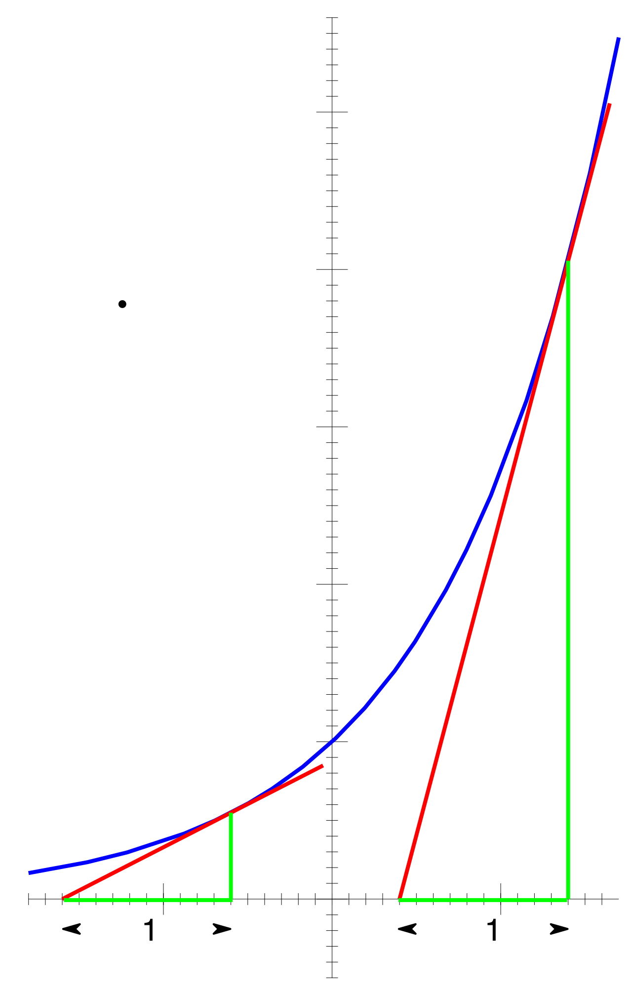
The natural exponential function is unique because it is its own derivative; the slope of its tangent line at any point equals the exact value of the function itself.

For other bases, we must adjust for the "stretch." The derivative of a general exponential function $a$ to the power of $x$ is $a$ to the power of $x$ multiplied by the natural logarithm of $a$ . $\frac{d}{dx}[a^x] = a^x \ln(a)$ For this to exist in the real number system, the base ' $a$ ' in the derivative formula for a general exponential function must be strictly greater than zero.

Logarithms

Logarithms unpack exponential growth. The derivative of the natural logarithm function $\ln(x)$ is the constant one divided by $x$ . $\frac{d}{dx}[\ln(x)] = \frac{1}{x}$ Because the natural logarithm is only defined for positive numbers, the domain of the derivative of the natural logarithm function $\ln(x)$ is all strictly positive real numbers.

However, if we take the absolute value, creating $\ln(|x|)$ , we mirror the graph into the second quadrant. The slopes on the left side perfectly match the formulation of the right. Thus, the derivative of the composite function $\ln(|x|)$ is the constant one divided by $x$ for all non-zero real numbers. This fact is incredibly important to remember when teaching integration later in the curriculum.

For logarithms of different bases, the derivative of a general logarithmic function log base $a$ of $x$ is the constant one divided by the product of $x$ and the natural logarithm of $a$ . $\frac{d}{dx}[\log_a(x)] = \frac{1}{x \ln(a)}$ Just as with exponentials, the base ' $a$ ' in the derivative formula for a general logarithmic function must be positive and not equal to one.

Logarithmic Differentiation

When faced with bizarre structural nightmares—like a variable in both the base and the exponent ( $x^{\sin(x)}$ )—standard rules fail. The power rule requires a constant exponent; the exponential rule requires a constant base.

Differentiating a function of the form $f(x)$ to the power of $g(x)$ mathematically requires the use of logarithmic differentiation. This is a brilliant algebraic workaround. Logarithmic differentiation involves taking the natural logarithm of both sides of an equation before applying implicit differentiation.

By utilizing the log property $\ln(A^B) = B \ln(A)$ , we pull the variable exponent down to the baseline, transforming an impossible power into a manageable product. Beyond variable exponents, logarithmic differentiation is a technique that simplifies the differentiation of functions containing complex products, quotients, or variable exponents. Taking the natural log transforms massive multiplications and divisions into simple addition and subtraction via logarithm properties, turning a grueling quotient-and-product rule marathon into a trivial sum.

The final major family of functions dictates harmonic motion and angles.

Here are the six standard trigonometric derivatives:

The derivative of the sine function is the cosine function. $\frac{d}{dx}[\sin(x)] = \cos(x)$
The derivative of the cosine function is the negative sine function. $\frac{d}{dx}[\cos(x)] = -\sin(x)$
The derivative of the tangent function is the square of the secant function. $\frac{d}{dx}[\tan(x)] = \sec^2(x)$
The derivative of the cotangent function is the negative square of the cosecant function. $\frac{d}{dx}[\cot(x)] = -\csc^2(x)$
The derivative of the secant function is the product of the secant function and the tangent function. $\frac{d}{dx}[\sec(x)] = \sec(x)\tan(x)$
The derivative of the cosecant function is the negative product of the cosecant function and the cotangent function. $\frac{d}{dx}[\csc(x)] = -\csc(x)\cot(x)$

The Radian Mandate

A severe and common pitfall for high school students involves units. Calculus rests heavily upon a specific limiting geometric argument: $\lim_{x \to 0} \frac{\sin(x)}{x} = 1$ . This limit is strictly, exclusively true if $x$ is measured in radians. Therefore, the argument of trigonometric functions must be measured in radians when applying standard trigonometric derivative formulas.

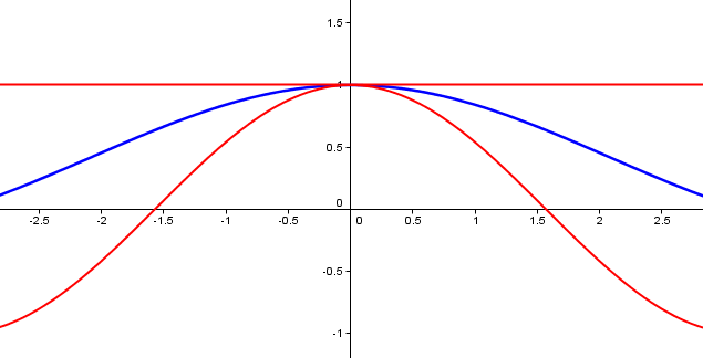
The foundational limit of sin(x)/x as x approaches 0, relying on this geometric squeeze theorem, is only valid when the angle x is measured in radians.

If a problem insists on degrees, calculus doesn't break, but it requires a chain-rule intervention. Applying standard derivative rules to trigonometric functions evaluated in degrees requires an additional scaling factor of $\pi$ divided by $180$ . If you are teaching a physics application where an angle $\theta$ is in degrees, $\frac{d}{d\theta}[\sin(\theta^\circ)] = \frac{\pi}{180}\cos(\theta^\circ)$ .

Inverse Trigonometric Derivatives

Inverse trigonometric functions ask us to find the angle when given a ratio. Their derivatives yield astonishingly neat algebraic fractions, free of any trigonometric operators. Understanding the domains of these derivatives is critical for exam success.

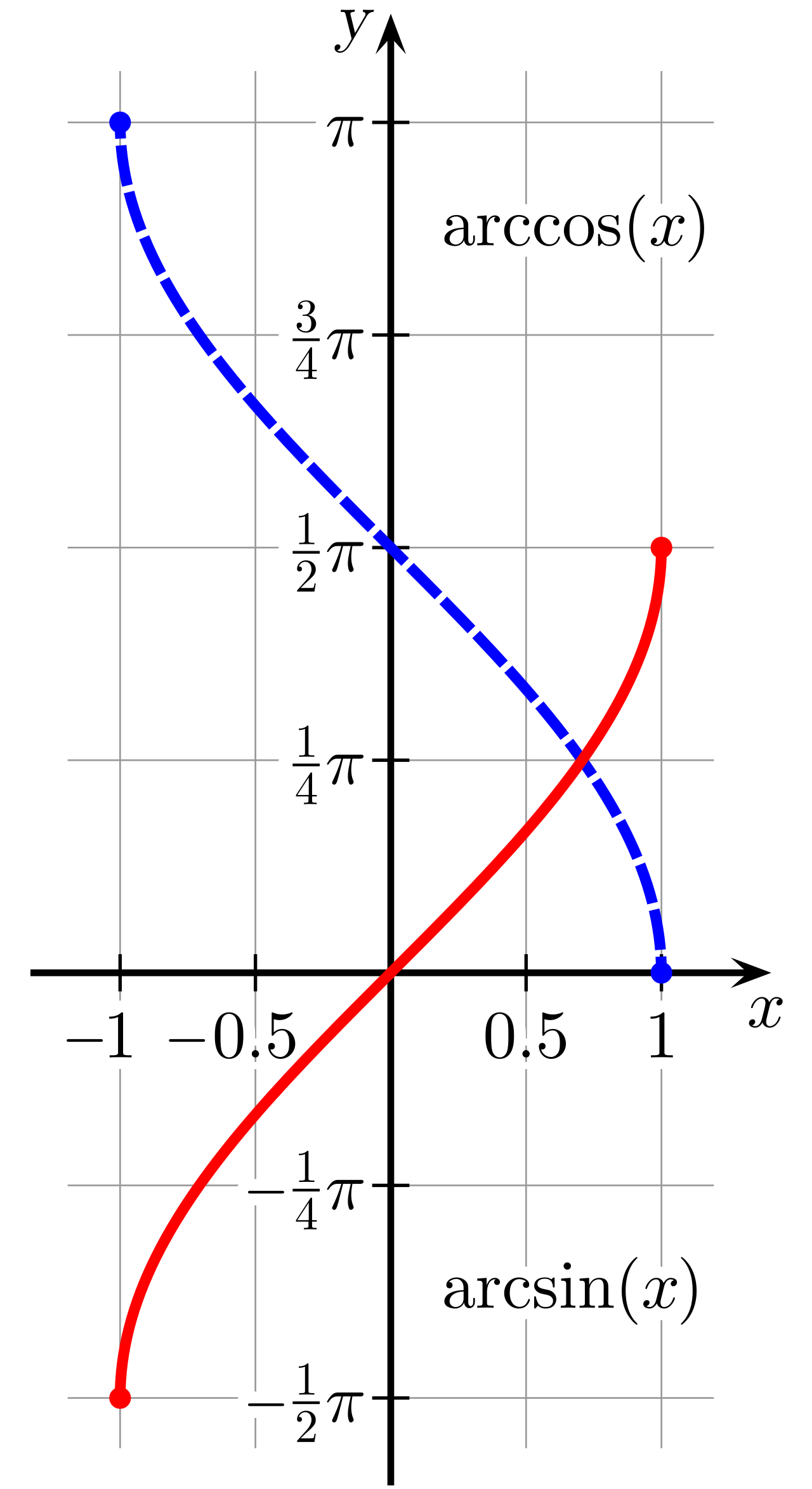
The derivative of the arcsine function is the constant one divided by the square root of the quantity one minus $x$ squared. $\frac{d}{dx}[\arcsin(x)] = \frac{1}{\sqrt{1-x^2}}$ Notice the denominator. If $x = 1$ or $x = -1$ , the denominator is zero. Even though the original arcsine function includes $-1$ and $1$ in its domain (endpoints of the curve), the tangent line goes vertical at these extremes. Therefore, the domain of the derivative of the arcsine function is the open interval from negative one to one $(-1, 1)$ .

The arccosine derivative is simply the negative of the arcsine derivative. The derivative of the arccosine function is negative one divided by the square root of the quantity one minus $x$ squared. $\frac{d}{dx}[\arccos(x)] = \frac{-1}{\sqrt{1-x^2}}$

The graphs of the arcsine and arccosine functions. Notice how their curves go completely vertical at x = -1 and x = 1, explaining why their derivatives are undefined at those endpoints.

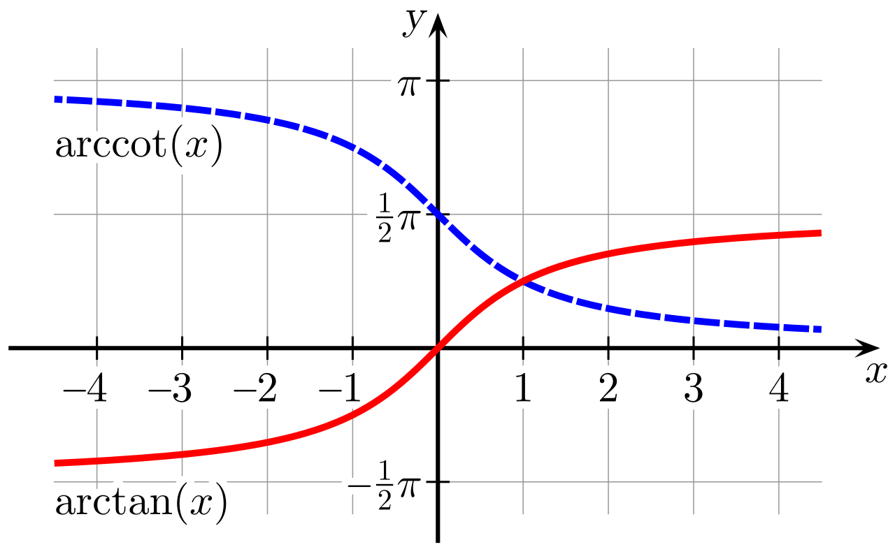
Finally, the arctangent, whose original graph spans infinitely across the x-axis, bounded horizontally by asymptotes at $\pm \frac{\pi}{2}$ . The derivative of the arctangent function is the constant one divided by the quantity one plus $x$ squared. $\frac{d}{dx}[\arctan(x)] = \frac{1}{1+x^2}$ Because the denominator $1+x^2$ can never be zero for any real number $x$ , there are no vertical tangents or breaks. Consequently, the domain of the derivative of the arctangent function is all real numbers.

Unlike arcsine, the arctangent function is bounded by horizontal asymptotes and possesses no vertical tangents, allowing its derivative to be valid for all real numbers.

When approaching the 5165 Mathematics exam, recognize that the test assesses both your procedural fluency and your pedagogical foresight. You are expected to instantly deploy the chain, product, and quotient rules. But more profoundly, you are expected to know why a student's graphing calculator shows a vertical asymptote in the derivative graph of $\arcsin(x)$ at $x=1$ , or why a student attempting to use the power rule on $x^x$ will arrive at mathematical nonsense.

Master the rules not just as abstract algorithms, but as precise tools for measuring reality—because that is the exact perspective you will need to impart to your future students.