Experimental Design and Analysis

Not sure you’re ready?

Take the ~3-minute readiness diagnostic and see where you stand.

Imagine trying to isolate exactly which string on a single violin is out of tune while a hundred-piece orchestra plays a roaring symphony. Biology is much like this. Organisms are infinitely complex, chaotic systems affected by a myriad of overlapping factors—temperature, genetics, nutrition, time, and environment all playing at once. To understand how life actually works, we cannot merely observe the noise; we must systematically silence the rest of the orchestra so we can listen to a single instrument. Experimental design is the architecture of that silence.

As a biology teacher, your goal is not just to teach students what we know about cells and ecosystems, but how we know it. Teenagers are natural, albeit flawed, empiricists. A student might drink a high-caffeine energy drink, try a new flashcard app, score an A on their biology exam, and conclude the energy drink is a cognitive enhancer. Teaching them the rigorous principles of experimental design equips them with a permanent intellectual filter. It allows them to separate truth from coincidence, signal from noise, and biology from marketing.

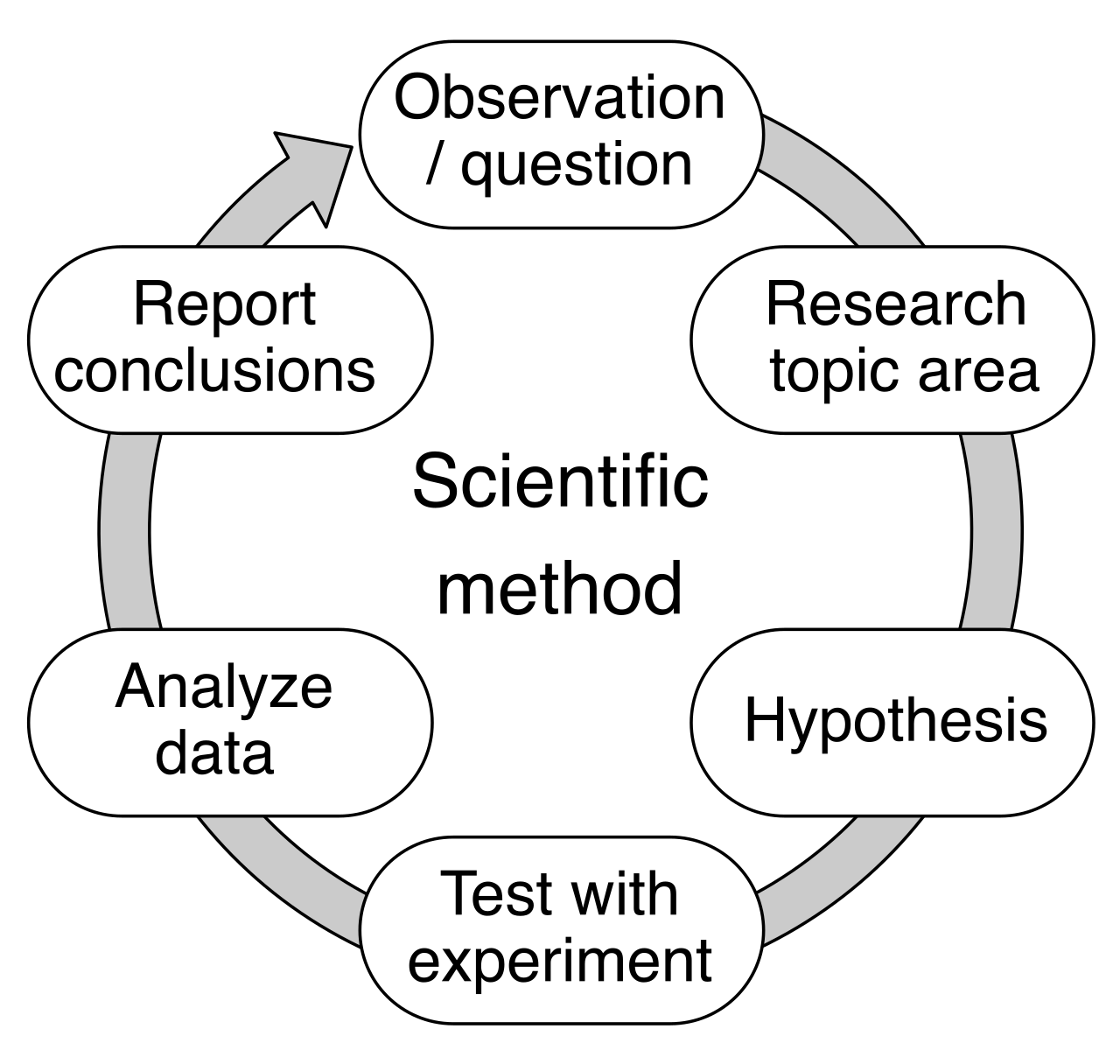
The scientific method is an iterative, structured process of observation, hypothesis formation, experimentation, and analysis used to filter out noise and discover biological mechanisms.

The foundation of any scientific investigation is a hypothesis, which is a testable and falsifiable proposed explanation for an observed scientific phenomenon. A statement like "Photosynthesis is beautiful" is a philosophical opinion; "Increased light intensity increases the rate of photosynthesis" is a hypothesis because we can test it, and crucially, we can prove it wrong.

However, in science, we must adopt a mindset of profound humility: a hypothesis cannot be proven absolutely true by experimental data. Experimental data can only support or reject a proposed hypothesis. There is always the possibility that an undiscovered mechanism is at play.

To formalize this testing, we establish two competing statements:

The null hypothesis: Proposes that there is no statistical relationship or effect between the independent and dependent variables. (e.g., "Light intensity has no effect on photosynthetic rate.")
The alternative hypothesis: Proposes that a specific relationship or effect exists between the independent and dependent variables.

To test these hypotheses, we must isolate the parts of the system, known as variables.

An independent variable is the specific condition deliberately manipulated by the researcher in an experiment. It is the cause.
A dependent variable is the measurable outcome or response observed during an experiment. It is the effect.
Controlled variables are baseline conditions kept exactly constant across all experimental groups (e.g., keeping the temperature, soil type, and plant species identical).
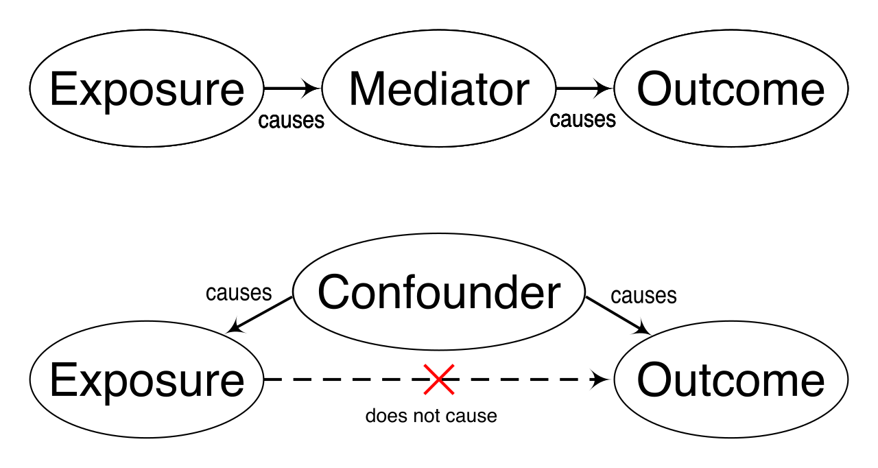
Confounding variables are unmeasured external factors that independently affect the dependent variable, secretly hijacking the experiment. If one greenhouse has a hidden draft, temperature becomes a confounding variable, making it impossible to tell if the light intensity or the cold air caused the plant's altered growth.

A confounding variable is an unaccounted external factor that independently influences the dependent variable, creating a false impression of a direct causal relationship.

A well-designed experiment must have a built-in reality check. How do we know our chemical reagents aren't spoiled? How do we know our spectrophotometer is working? We use control groups.

A negative control group is exposed to all experimental conditions except the treatment expected to produce an effect. If you are testing a new antibiotic, the negative control is a bacterial plate given no antibiotic. If bacteria die here anyway, your baseline is flawed.
A positive control group receives a treatment already known to produce a specific measurable effect. If you use a standard, well-documented antibiotic on another plate, and the bacteria don't die, your bacteria are invincible or your agar is wrong. Ultimately, positive control groups validate that the experimental measurement system is functioning properly.

When dealing with complex organisms—especially humans or highly variable ecological plots—we must account for inherent diversity. We use random assignment, which minimizes preexisting differences between subjects in experimental and control groups. We also rely heavily on replication, which involves repeating an experiment on multiple independent subjects or under identical conditions. A single plant dying means nothing; a thousand plants dying is a pattern. Replication increases the statistical reliability of experimental results.

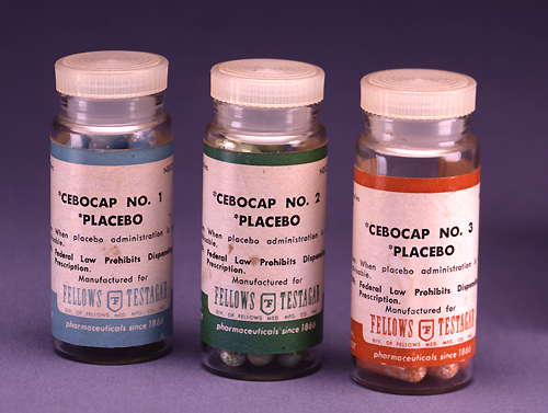
In human trials, psychology introduces a powerful confounding variable: expectations. To combat this, we use a double-blind study, which prevents both the human subjects and the researchers from knowing which specific treatment group participants belong to. Double-blind studies reduce the impact of researcher bias and the placebo effect on experimental outcomes, ensuring that the biological effect is genuine.

In clinical trials, placebos—such as inert sugar pills—are administered to control groups to account for the psychological impact of a subject's expectations.

Science requires a universal language. If a Russian botanist, a Brazilian ecologist, and an American geneticist compare notes, they cannot be arguing over ounces and inches.

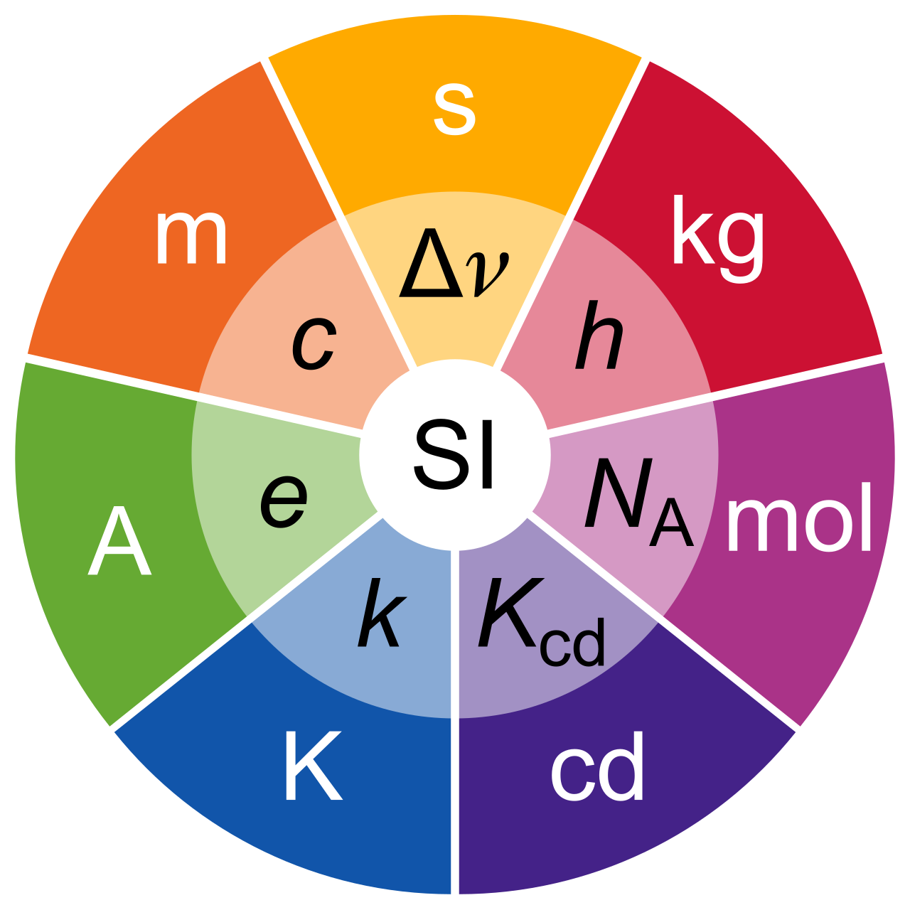
The International System of Units (SI) is the globally accepted standard metric system for scientific measurements. As you prepare secondary students for lab work, they must internalize its foundations:

The base unit for measuring mass is the kilogram.
The base unit for measuring length is the meter.
The base unit for measuring time is the second.
The base unit for measuring the amount of a chemical substance is the mole.
The base unit for measuring thermodynamic temperature is the kelvin.

The International System of Units (SI) provides a coherent, globally recognized framework of base units that allows scientific measurements to be universally communicated and replicated.

To translate between scales—say, from grams to kilograms or seconds to years—we use dimensional analysis, a mathematical method for converting between different units of measurement using conversion factors. A conversion factor is a ratio of equivalent measurements expressed in two different units (like $1 \text{ kg} / 1000 \text{ g}$ ).

The beauty of dimensional analysis is that measurement units are treated as algebraic quantities that can be multiplied and canceled out. If a student sets up the equation correctly, the unwanted units disappear like common variables in an algebra fraction, leaving only the desired metric behind.

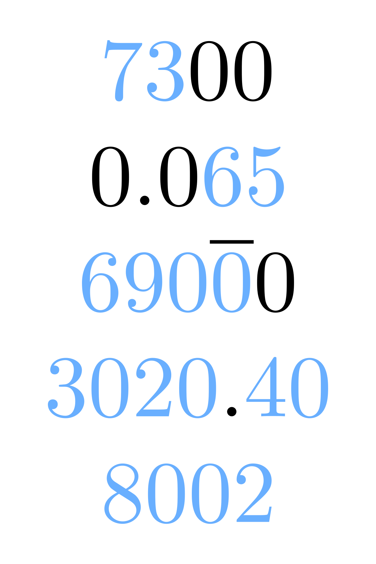
In a math class, $3.0$ and $3$ are identical. In a biology lab, they are entirely different statements about reality. Numbers in science carry the physical limitation of the tool used to measure them. Significant figures indicate the precision of a measured physical quantity. Writing $3.00 \text{ g}$ tells the world, "I used a scale capable of reading hundredths of a gram."

To read and write the language of significant figures, we follow strict rules:

All non-zero digits in a measured scientific value are always considered significant figures. (e.g., $452$ has three).
Zeroes located exactly between two non-zero digits are always considered significant figures. (e.g., $4002$ has four).
Leading zeroes located at the beginning of a decimal number are never considered significant figures; they are merely placeholders. (e.g., $0.005$ has only one).
Trailing zeroes in a number containing a written decimal point are always considered significant figures. (e.g., $4.500$ has four).

Significant figures visually identified: leading zeroes simply locate the decimal point and are not significant, while non-zero digits and trailing zeroes represent genuine measurement precision.

When we manipulate these measurements mathematically, the resulting number cannot magically become more precise than the weakest link in our data.

When multiplying or dividing measurements, the final answer must have the exact same number of significant figures as the original measurement with the fewest significant figures.
When adding or subtracting measurements, the final answer must have the exact same number of decimal places as the original measurement with the fewest decimal places.

Imagine throwing darts at a dartboard.

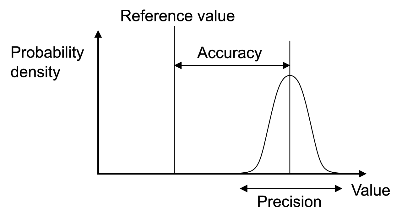
Accuracy describes how close a measured value is to the true or universally accepted value. (Hitting the bullseye).
Precision describes how closely repeated independent measurements agree with one another. (Hitting the exact same spot on the wall three times, even if it's far from the bullseye).

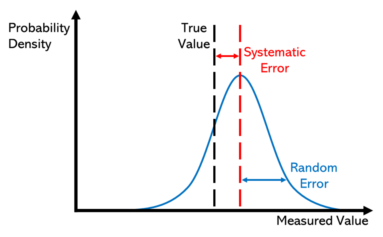
High accuracy means measurements are close to the true value, while high precision means repeated measurements are clustered closely together, regardless of their accuracy.

When a student misses the "true" biological value, it is due to error. But not all errors are created equal.

Systematic errors consistently shift all measured values in the exact same direction away from the true value. They skew the data left or right across the board. These often result from improperly calibrated laboratory equipment—like a pipette that always delivers 0.1 mL less than the dial indicates. Because it skews the reality of the data, systematic errors directly reduce the accuracy of an experiment. Crucially, increasing the sample size of an experiment does not reduce the impact of systematic error. Measuring a thousand incorrect volumes still yields an incorrect average.

Conversely, random errors are unpredictable measurement variations that scatter data equally above and below the true value. Perhaps a student's hand shakes slightly while reading a meniscus. Because the measurements scatter, random errors directly reduce the precision of an experiment. However, because they fluctuate randomly high and low, they tend to cancel each other out over time. Therefore, increasing the sample size reduces the mathematical impact of random error on the average experimental result.

Systematic errors shift the entire distribution of data away from the true value, while random errors scatter the data, widening the distribution without inherently shifting its center.

Once the data is collected, we must decide what it means. Raw data is messy.

First, we look at the spread. Standard deviation measures the total amount of variation or dispersion within a set of recorded data points. A high standard deviation means the data is widely scattered; a low standard deviation means the data points are tightly clustered around the mean.

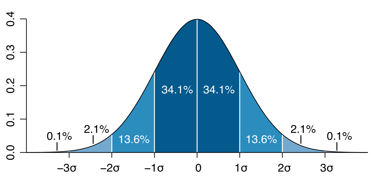
Standard deviation measures data dispersion. In a normal distribution, roughly 68% of the data points cluster within one standard deviation (dark blue) of the mean.

Next, we calculate our confidence in our findings. The standard error of the mean estimates how closely a calculated sample mean matches the true population mean. When you graph data, you don't just plot dots; you plot an average with "whiskers" sticking out of it. These error bars on a scientific graph visually represent the statistical variability or uncertainty of the reported data.

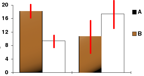
Error bars visually represent the statistical uncertainty of an average. They are vital for interpreting whether observed changes are genuine biological responses or just statistical noise.

If you compare the heights of two plant groups, and the error bars cross each other's paths, the noise of the data is louder than the signal. Overlapping error bars on a graph typically indicate that the numerical difference between two means is not statistically significant.

To make a final judgment, biologists use inferential statistics to calculate a p-value, which calculates the exact probability of obtaining the observed experimental results assuming the null hypothesis is completely true. If a p-value is 0.03, it means there is only a 3% chance we would see these results if the independent variable actually had no effect.

The standard significance level used in most biological research is 0.05.

A p-value strictly less than the predetermined significance level indicates that the experimental results are statistically significant.
These statistically significant experimental results lead researchers to formally reject the null hypothesis.

The Golden Rule: Correlation vs. Causation

We end with a vital warning for your future students. Suppose you find a p-value of 0.01 showing a strong link between ice cream sales and shark attacks. You reject the null hypothesis. Does ice cream summon sharks? No. Both are independently caused by a confounding variable: warm summer weather.

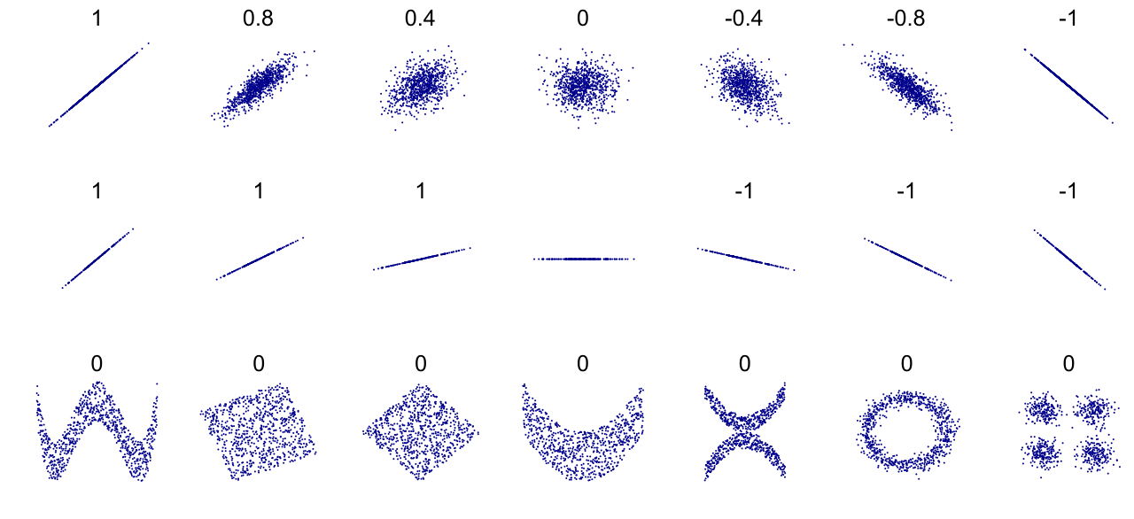
A strong mathematical correlation between two variables does not prove that one variable causes the change in the other. Experimental design, strict controls, and logical isolation of variables are the only ways to bridge the gap between noticing a pattern and proving a mechanism. Mastering these principles transforms students from passive consumers of information into rigorous, scientific thinkers.

Datasets can display varying degrees of mathematical correlation. However, even a robust correlation coefficient (such as 1.0) cannot on its own prove that one variable causes the other.