Measures of Spread: Range and Standard Deviation

Not sure you’re ready?

Take the ~3-minute readiness diagnostic and see where you stand.

Imagine evaluating the climate of two different cities that both boast an average annual temperature of 65 degrees Fahrenheit. One city experiences a mild, perpetual spring, fluctuating merely between 60 and 70 degrees year-round. The other city suffers scorching 100-degree summers and freezing 30-degree winters. A single number—the average—fails completely to capture the reality of living in either location. To understand the true nature of a collection of numbers, we must look beyond the center and examine the periphery. We must measure the variation. Measures of spread describe how varied the values are within a single data set. They are the mathematical tools that distinguish the predictably consistent from the wildly erratic.

For future educators, understanding this variation is just as vital as understanding the average. If a class averages 75% on an exam, the instructional response changes drastically depending on whether every student scored exactly 75%, or half the class scored 100% while the other half scored 50%. The measures of spread guide those pedagogical decisions.

When we first attempt to measure how spread out our data is, the most intuitive approach is to look at the outer boundaries. How wide is the entire data set from start to finish? This gives us our simplest measure of spread.

Definition: The range of a data set is the difference between the maximum value and the minimum value.

$\text{Range} = \text{Maximum} - \text{Minimum}$

In practice, a student calculates the range by subtracting the minimum value from the maximum value in a data set. If the highest score on a math quiz is 98 and the lowest score is 42, the range is $98 - 42 = 56$ . Because this calculation simply subtracts two values from the data set, the range is expressed in the exact same units as the original data values. If we are measuring student heights in inches, the range is measured in inches. If we are tracking textbook costs, the range is measured in dollars, such as a difference of $45.

The Fatal Flaw of the Range

While simple to compute, the range has a severe limitation: the calculation of the range relies exclusively on the two extreme values of a data set. It completely ignores everything happening in the middle.

Consider a classroom where 19 students score between 85% and 90% on a test, but one student, who was absent for a week, scores a 12%. Because the range relies entirely on the extremes, the range is highly sensitive to outliers. The presence of that single 12% will artificially inflate the range to $90 - 12 = 78\%$ , falsely suggesting a massively varied classroom performance when, in reality, almost the entire class performed uniformly.

To construct a mathematically robust picture of variation, we cannot simply look at the edges of the data. We must account for every single data point and ask: on average, how far away is each data point from the center?

This brings us to the most important concept in data variability. Standard deviation measures the typical distance of individual data points from the mean of the data set.

Imagine the mean (the average) as a campfire, and the data points as people sitting around it. Standard deviation simply asks: on average, how far away from the fire is everyone sitting?

A low standard deviation indicates that the data points tend to be clustered closely around the mean. (Everyone is huddled tight around the campfire).
A high standard deviation indicates that the data points are spread out over a wide range of values. (People are scattered randomly throughout the campsite).

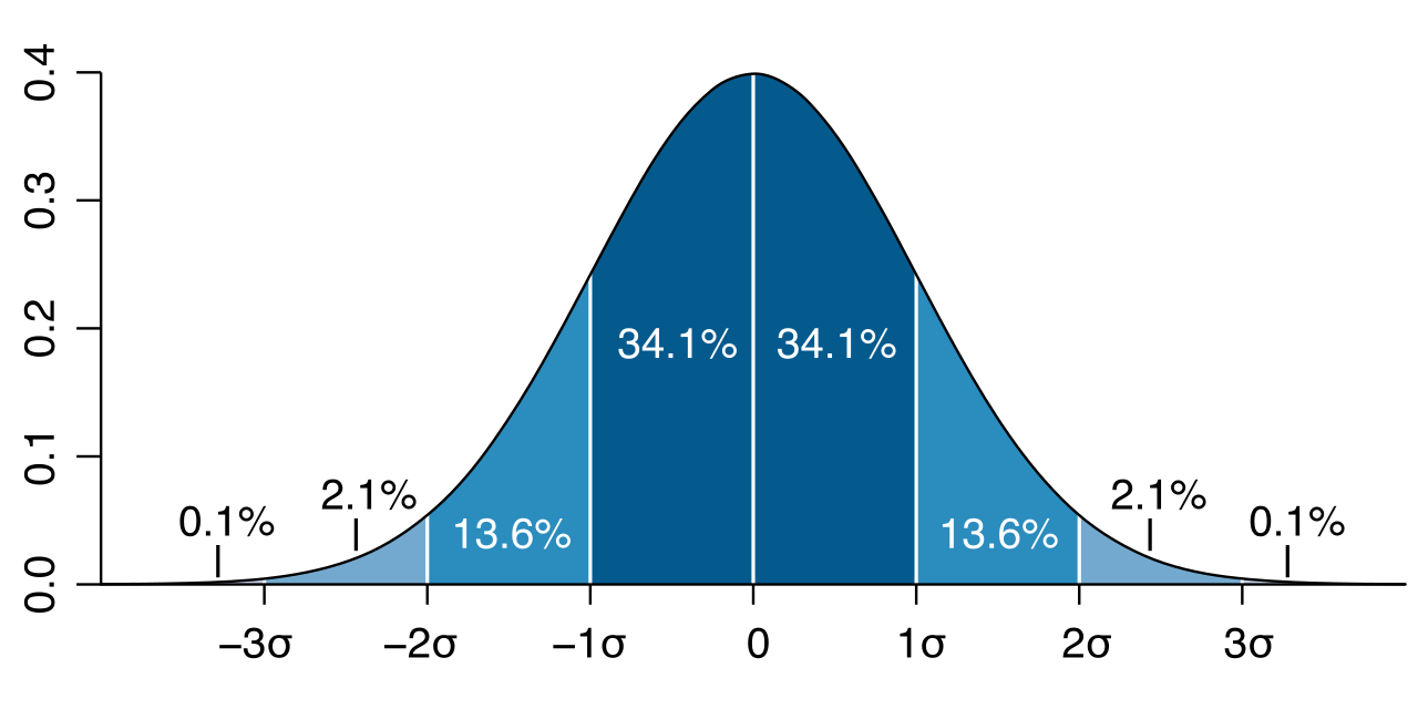
Standard deviation visualizes the typical dispersion of data points around the mean. In a normal, bell-shaped distribution, the vast majority of the data clusters within one or two standard deviations of the center.

Like the range, standard deviation is grounded in physical reality; standard deviation is expressed in the exact same units as the original data values. If you are calculating the standard deviation of test scores, your standard deviation is in "points."

The Mathematical Rules of Standard Deviation

Because standard deviation represents a physical distance from a central point, it is subject to the rules of absolute distance.

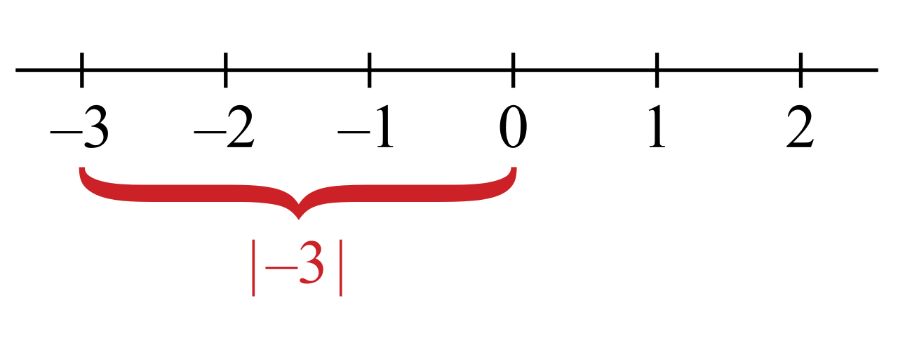
Because it represents physical distance, standard deviation behaves conceptually like absolute value—it measures magnitude away from a center point and can never be negative.

It is always positive or zero: Standard deviation can never be a negative number. You cannot have a negative distance between a data point and the mean.
The meaning of zero: What happens if the standard deviation is zero? A standard deviation of exactly zero means that every single value in the data set is identical. There is no spread whatsoever. If every student in a class scores an 85 on an exam, the mean is 85, and the distance of every score from that mean is zero.
The impact of extremes: While standard deviation utilizes every data point (unlike the range), it is still affected by extreme values. Because distances are squared during its mathematical calculation (to prevent negative distances from canceling out positive ones), adding an extreme outlier to a data set increases the standard deviation of that data set, pulling that "typical distance" upward.

Educators frequently use standard deviation to compare different classes, different exams, or different instructional methods. Standard deviation provides a reliable metric for consistency.

Two distinct sets of data can share the exact same mean but exhibit vastly different standard deviations. The wider distribution indicates greater variability and lower consistency among the data points.

Data Set characteristic	Interpretation	Example in a Classroom Context
Larger Standard Deviation	When comparing two data sets, the data set with the larger standard deviation exhibits greater overall variability.	Class A has a mean of 75 and a standard deviation of 15. The scores are widely varied; some students failed, while others excelled.
Smaller Standard Deviation	When comparing two data sets, the data set with the smaller standard deviation exhibits greater overall consistency.	Class B has a mean of 75 and a standard deviation of 3. Almost every student scored firmly between 72 and 78.

If you are trying to determine whether a new teaching intervention worked uniformly for everyone, you want to see a smaller standard deviation. A smaller standard deviation means the intervention produced a consistent effect, whereas a larger standard deviation means the intervention worked wildly differently for different students.

A frequent topic on the Praxis Core involves understanding how mathematical operations applied to an entire data set affect the measures of spread. Let's explore the geometry of transforming data.

Shifting Data (Addition and Subtraction)

Suppose an exam was unexpectedly difficult, and the teacher decides to curve the grades by adding 5 bonus points to every student's score.

Visualize this on a number line. Every single data point picks up and moves 5 units to the right. The entire shape of the data curve remains identical; it has simply slid down the axis. Because the distance between the maximum and minimum values does not change, adding a constant value to every number in a data set does not change the range of the data set.

When data is shifted by adding or subtracting a constant, the entire distribution simply slides along the number line, leaving the measures of spread entirely unchanged.

Similarly, the distance between any individual point and the new mean remains exactly the same as it was before the shift. Therefore, adding a constant value to every number in a data set does not change the standard deviation of the data set.

Rule of Thumb: Shifting data changes the location (mean, median), but it never changes the spread (range, standard deviation).

Scaling Data (Multiplication and Division)

Now suppose a quiz was graded out of 50 points, and the teacher wants to convert the scores to percentages out of 100. To do this, the teacher multiplies every student's score by $2$ .

If the original maximum was 45 and the minimum was 30, the original range was $15$ . After multiplying by $2$ , the new maximum is 90 and the new minimum is 60. The new range is $30$ . The spread has been stretched like a rubber band. Multiplying every number in a data set by a positive constant multiplies the range by that exact same constant.

Because the entire data set has been stretched apart, the distance of each data point from the mean has also been stretched by a factor of 2. Therefore, multiplying every number in a data set by a positive constant multiplies the standard deviation by that exact same constant.

While standard deviation is highly intuitive because it shares the same units as the original data, statisticians sometimes rely on a related sibling metric during calculations.

Variance is defined mathematically as the square of the standard deviation.

If the standard deviation of a set of test scores is $4$ points, the variance is $16$ "squared points." While "squared points" are incredibly difficult to interpret intuitively in the real world (which is why standard deviation is preferred for practical reporting), variance is foundational for higher-level statistics because it removes negative signs from algebraic proofs seamlessly. Whenever you need the variance, simply square the standard deviation; if you have the variance and need the standard deviation, take the square root.