Random Sampling and Population Inferences
Not sure you’re ready?
Take the ~3-minute readiness diagnostic and see where you stand.
Imagine a chef preparing a massive vat of soup for a banquet. To determine if the broth requires more salt, the chef does not need to consume the entire 50-gallon vat. Instead, they stir the pot thoroughly and draw a single spoonful. That single spoonful reveals the flavor profile of the entire batch. This intuitive act captures the essence of statistical sampling. We extract a manageable piece of a whole, observe its properties, and boldly extrapolate those properties back to the enormous, unknowable whole. In mathematics, this process transitions from culinary intuition into a rigorous, verifiable methodology.
To think clearly about statistics, we must first define the boundaries of our universe of inquiry. A population is the entire group of individuals or objects of interest in a statistical study. It is the whole vat of soup. It is every registered voter in a country, every lightbulb produced in a factory on a Tuesday, or every student enrolled in a vast university system.
Because measuring every individual in a population of millions is often financially and logistically impossible, we rely on a sample, which is a smaller subset of individuals selected from a larger population. We analyze the sample not because we care exclusively about those few individuals, but because we care about what they represent. The logical leap from that small subset to the grand whole is known as making statistical inferences—mathematical conclusions drawn about an entire population based on data collected from a sample.
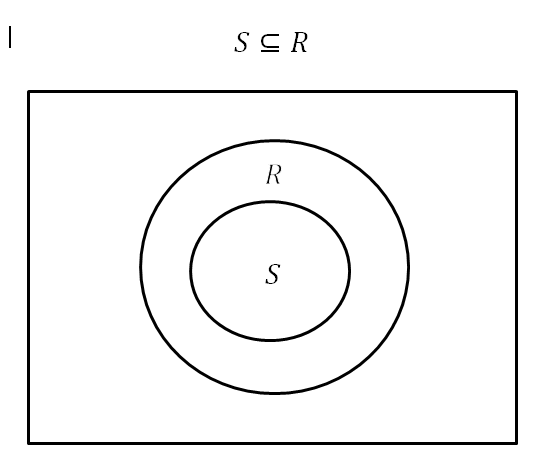
For an inference to be logically sound, the sample must look like the population in miniature. A representative sample accurately reflects the true characteristics of the overall population. If the population is 60% female, the sample should be roughly 60% female; if 20% of the population is left-handed, the sample should mirror that trait.
How do we ensure our sample is perfectly representative? We surrender control to probability.
Random sampling is a selection method where every member of the population has an equal probability of being chosen. This is the cornerstone of statistical science because random sampling minimizes selection bias. When human beings hand-pick a sample, conscious and unconscious preferences infect the data. When chance dictates the sample, the mathematical laws of probability ensure a balanced reflection of the whole.
When we fail to utilize randomness, we often create a biased sample, which forms when a selection process favors certain members of a population over others. Crucially, statistical inferences derived from a biased sample inaccurately represent the total population. If you want to study the study habits of university students, but you only sample students found in the library at midnight on a Friday, your inferences will be hopelessly skewed.
Once we possess a truly random, representative sample, we can begin making calculations. The most vital calculation for this purpose is the sample proportion.
A sample proportion is calculated by dividing the number of individuals in a sample with a specific trait by the total sample size.
Sample Proportion=Total Sample SizeIndividuals with a Specific Trait
This resulting decimal or fraction is far more than a mere descriptor of the sample. A sample proportion serves as the mathematical estimate for a specific trait's prevalence within an entire population.
If we survey 400 randomly selected teachers in a state and find that 100 of them hold a master's degree, our sample proportion is: 100÷400=0.25
We now possess the mathematical estimate (25%) for the prevalence of master's degrees among all teachers in the state.
Scaling to the Population
Crucial Exam Insight: The Praxis Core Mathematics exam requires test-takers to scale a sample proportion up to a predicted total population count.
Predicting a total population count for a specific trait requires multiplying the sample proportion by the total population size. The formula is remarkably straightforward:
Predicted Total Count=Sample Proportion×Total Population Size
Let's walk through an example: Suppose a district employs 8,000 teachers. Based on our random sample of 400 teachers where 100 had master's degrees (a sample proportion of 0.25), how many teachers in the entire district can we predict hold a master's degree?
Predicted Count=0.25×8000 Predicted Count=2000
We can reasonably infer that 2,000 teachers in the district hold a master's degree.
Not all random sampling is conducted by pulling names from a giant hat. Statisticians have engineered sophisticated methods to introduce randomness depending on the geographic and logistical realities of the population.
1. Simple Random Sample
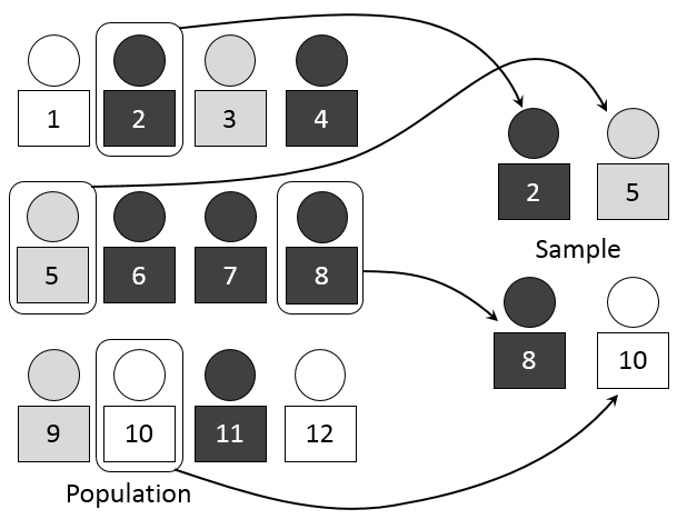
The purest, most foundational technique. A simple random sample ensures that every possible group of a specific size has an identical probability of selection. Imagine a lottery drum filled with ping-pong balls. Drawing 50 balls simultaneously gives every possible combination of 50 balls an equal mathematical chance of emerging.
2. Stratified Random Sampling
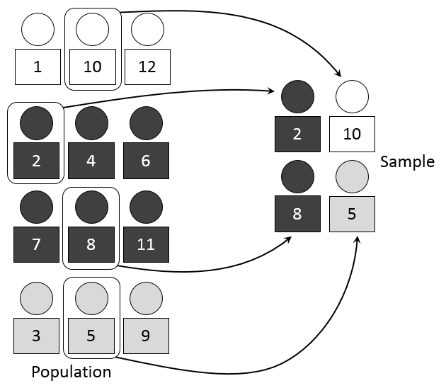
Sometimes, a population has distinct layers, and we want to guarantee that every layer is represented accurately. Stratified random sampling divides a population into distinct homogeneous subgroups (known as strata). Think of a high school divided cleanly into freshmen, sophomores, juniors, and seniors.
After drawing these boundary lines, stratified random sampling selects random individuals proportionally from predefined homogeneous subgroups. If the school is 30% freshmen, your sample will be engineered to be precisely 30% randomly selected freshmen.
3. Cluster Sampling
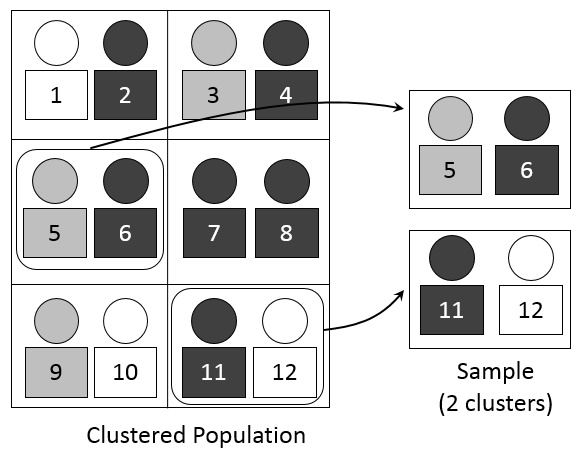
When a population is spread out over a massive area, random sampling can be impossibly expensive. Cluster sampling divides a population into distinct separate groups (clusters), such as individual classrooms in a large school district or city blocks in a metropolis.
Instead of randomly picking one person from every single group, cluster sampling randomly selects entire predefined groups to form a statistical sample. If you select Classroom A and Classroom D, you interview every single student in those specific rooms, and ignore the other rooms entirely.
4. Systematic Sampling
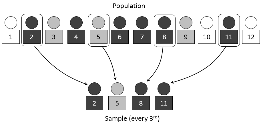
Often used in manufacturing or long rosters. Systematic sampling selects individuals at a regular numerical interval from a randomized population list. You might select every 15th lightbulb coming off an assembly line, or every 10th student on an alphabetical district roster, after starting at a random, randomly generated point (like the 7th name).
Stratified vs. Cluster Sampling
Students frequently confuse Stratified and Cluster sampling. Use this table to differentiate them conceptually:
| Feature | Stratified Random Sampling | Cluster Sampling |
|---|---|---|
| Division | Population divided into homogeneous groups based on a trait (e.g., Grade Level). | Population divided into distinct separate groups, usually geographically (e.g., Classrooms). |
| Selection | Randomly select individuals from all groups. | Randomly select some entire groups, ignoring the rest. |
| Goal | To guarantee proportional representation of specific subgroups. | To reduce logistical effort and cost while maintaining randomness. |
The beauty of mathematical inference collapses entirely if the data is gathered using flawed, non-random methods. Two common culprits routinely destroy the validity of statistical studies.
Convenience Sampling
Convenience sampling is a non-random selection method involving individuals who are most readily accessible to a researcher. Imagine a principal wanting to gauge the entire student body's interest in a new dress code, but they only ask the students sitting in the front row of the cafeteria during the first lunch period. Because it ignores the vast majority of the population based purely on ease of access, convenience sampling routinely introduces severe selection bias into statistical data.
Voluntary Response Sampling
Voluntary response sampling occurs when individuals self-select to participate in a statistical study. Internet polls, call-in radio shows, and mailed surveys with no follow-up are classic examples.
Human nature dictates a fundamental flaw here: voluntary response sampling generally attracts individuals with strong opinions. People who are mildly indifferent do not take the time to call a radio station or fill out a web form. Because the resulting group is hyper-concentrated with extreme viewpoints (either highly positive or highly negative), voluntary response sampling reliably introduces selection bias into statistical datasets.
Even when we execute a flawless Simple Random Sample, we must maintain intellectual humility. If I randomly sample 100 students and find that 42% prefer remote learning, and you independently sample 100 random students from the same school, you might find that 45% prefer remote learning.
Who is wrong? Neither of us.
Sampling variability describes the phenomenon where different random samples drawn from the same population yield slightly different mathematical results. This is the natural static of the mathematical universe. Because we are looking at subsets and not the whole, minor fluctuations are inevitable.
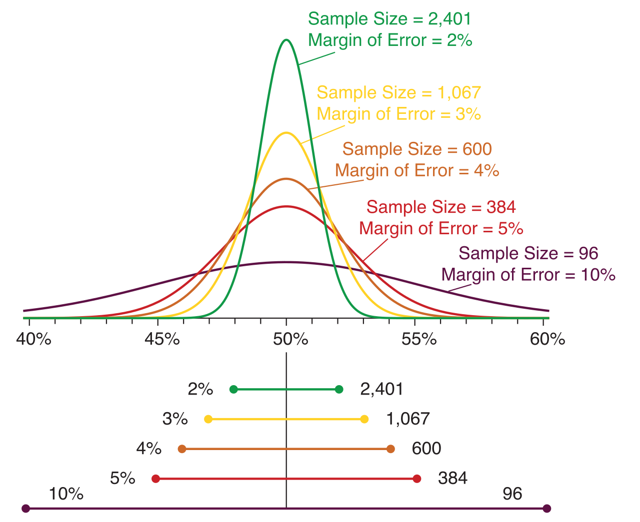
Because of sampling variability, we rarely state statistical inferences as absolute certainties. Instead, we use a buffer. The margin of error defines the expected numerical deviation between a calculated sample statistic and an actual population parameter. You will commonly see this in polling: "42% of voters support the measure, with a margin of error of plus or minus 3 percentage points." This tells us the true population parameter is highly likely to reside somewhere between 39% and 45%.
If we wish to shrink our uncertainty and paint a sharper picture of reality, we have one reliable mathematical lever to pull: sample size. Increasing the sample size reduces the margin of error in population estimates. A random sample of 10 individuals is highly susceptible to a single outlier warping the proportion. A random sample of 1,000 individuals exerts a massive gravitational pull, drowning out the outliers and pulling the sample proportion remarkably close to the absolute truth of the entire population.