Education needs analysis
Imagine calculating the trajectory of an interceptor missile aiming for a target that is simultaneously moving away from you and accelerating at its own unique, highly aggressive rate. This is the exact physics of education needs analysis. When a client tells you they want to fully fund their toddler’s future college education, you are not merely solving a static present value problem. You are solving for a future liability that is subject to a specialized rate of inflation, requiring a lump sum at a highly specific point in time, which will be drawn down in an environment where the remaining principal continues to grow while the tuition costs continue to inflate. For the financial planner, mastering this architecture is not just about memorizing keystrokes on an HP-12C; it is about grasping the mechanics of purchasing power over time.
When we look at the cost of higher education, we must first abandon the assumption that general inflation applies. Historical education inflation has consistently outpaced the general economic inflation rate. If the Consumer Price Index is hovering around 2% to 3%, tuition costs have historically compounded at 5% to 6% or more. Therefore, the future cost of education must be projected using an expected education inflation rate rather than the general inflation rate. Using general inflation to project college costs is a mathematical guarantee that your client will underfund their goal.
To begin our calculation, we must determine exactly how much the first year of college will cost on the day the student steps onto campus.
Calculating Year One: The future value of the first year of college tuition is calculated using the time remaining until enrollment as the number of compounding periods (N).
If a child is 5 years old and will enroll at age 18, we have exactly 13 years of compounding before the first tuition check is cut. We inflate today’s current annual cost at the education inflation rate for 13 periods to find the cost of Freshman year.
College is rarely a single year. It is a multi-year liability. However, we do not simply add up the cost of four inflated years. Why? Because the money earmarked for Sophomore, Junior, and Senior years will remain invested, earning a return, even as tuition costs continue to inflate.
To determine the exact pile of capital needed on the first day of Freshman year, we must discount all expected future tuition payments back to a single present value. This introduces two critical rules of the education funding framework.
Rule 1: The Timing of Cash Flows
In the real world, universities do not let you attend classes and pay at the end of the year. College tuition payments are typically due and paid at the beginning of the academic year.
Because the first payment happens immediately on day one, financial calculators must be set to Begin or Annuity Due mode when calculating the present value lump sum required at the exact start of college. If you leave your calculator in "End" mode, you mathematically assume the money sits in the market earning a full year of interest before the first tuition bill is paid, resulting in a dangerously underfunded goal.
Rule 2: The Inflation-Adjusted Rate of Return
Because the tuition liability is inflating simultaneously as the invested assets are generating returns, we cannot discount the cash flows using the nominal investment return alone. An inflation-adjusted rate of return is required to discount future inflating tuition payments back to a present value at the start of college.
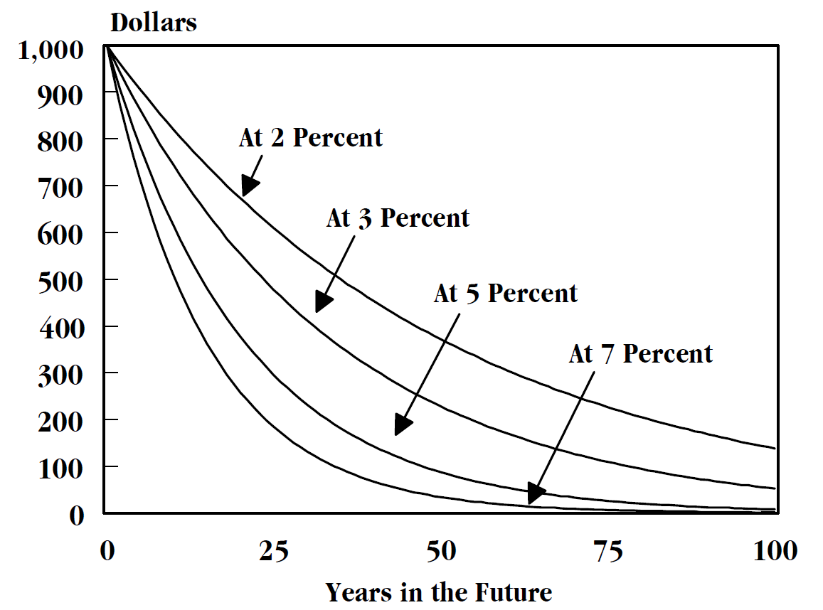
This rate represents the real growth of the money—the spread between the investment engine pushing the balance forward and education inflation dragging the purchasing power backward.
The Inflation-Adjusted Return Formula: Real Rate=[1+Inflation Rate1+Investment Return]−1×100 The formula for the inflation-adjusted rate of return is the investment return plus one divided by the inflation rate plus one minus one.
By using this adjusted rate, the total lump sum needed at the start of college is the present value of all expected tuition payments discounted at the inflation-adjusted rate.
Once we have determined the lump sum needed on enrollment day, the paradigm shifts. The calculated lump sum needed at the start of college serves as the future value goal for the savings accumulation phase.
Now, we must look at the time remaining until enrollment and determine what periodic deposits the parents must make today. The fundamental constraints of compounding apply here just as they do in retirement planning: higher expected investment returns during the accumulation phase reduce the required periodic savings amount for education funding. Conversely, a shorter accumulation period requires higher periodic savings contributions to reach the exact same education funding goal. Time is the most powerful lever in the equation.
When designing the savings schedule, the planner can structure the cash flows in two primary ways:
Fixed Level Payments
Level payment funding requires saving the exact same nominal dollar amount each period.
If the calculation determines a need of \$500 per month, the client pays exactly \$500 per month from today until enrollment. This is easy to automate and budget, but it can be intensely burdensome for young parents whose incomes are currently at the lowest point of their earning trajectory.
Increasing Serial Payments
Serial payment funding requires saving an amount that increases each period by a specified growth rate (typically mirroring the parents' expected salary growth or general inflation).
In year one, they might save \$400 per month. In year two, \$420. This structure allows younger families to begin funding earlier with a lighter initial burden. From a mathematical standpoint, serial payment calculations use the inflation-adjusted rate of return to determine the required savings amount for the very first period. By discounting both the final goal and the payment stream by the growth rate, you isolate the required purchasing power of the very first payment today.
Calculator Mechanics for Accumulation
The mechanics of how clients actually save money dictates your calculator settings.
- The accumulation phase calculation typically assumes regular savings deposits are made at the end of each period using ordinary annuity mode. Most clients save out of their paychecks at the end of the month or year.
- However, if savings contributions will be made at the beginning of each period, the financial calculator must be set to annuity due mode for the accumulation phase.
Furthermore, education funding is rarely done via annual lump sums. Most clients save monthly. Monthly education funding calculations require dividing the annual nominal interest rate by twelve and multiplying the total number of accumulation years by twelve to find the total periods.
Up to this point, we have assumed the client is fully funding 100% of the cost. But the reality is that the actual required funding is heavily influenced by the federal student aid environment. Understanding the architecture of the Free Application for Federal Student Aid (FAFSA) is paramount.
The Free Application for Federal Student Aid is the official form used to calculate eligibility for federal student financial aid.
The entire financial aid calculation hinges on one foundational equation:
Financial Need = Cost of Attendance (COA) - Student Aid Index (SAI) A student's financial need is calculated by subtracting the Student Aid Index from the official Cost of Attendance.
Let us break down these two variables.
The Cost of Attendance (COA)
The COA is a standardized statutory figure provided by the institution. It is not just the price of classes. The Cost of Attendance includes tuition, fees, room, board, books, transportation, and personal expenses. Naturally, any scholarships and grants reduce a student's out-of-pocket Cost of Attendance without requiring repayment, acting as a direct reduction to the family's required funding goal.
The Student Aid Index (SAI)
In a sweeping legislative update, the Student Aid Index replaced the Expected Family Contribution (EFC) metric for federal student aid calculations starting in the 2024-2025 award year. The SAI is an evaluation of the family's financial strength.
The federal formula heavily penalizes assets held in the student's name, expecting them to utilize more of their own net worth for school than the parents. Consider this profound asymmetry in the formula:
- Parent-owned 529 plan assets are assessed at a maximum rate of 5.64 percent in the Student Aid Index calculation.
- Student-owned assets are assessed at a 20 percent rate in the Student Aid Index calculation.
If a family holds \$10,000 in a parent-owned 529 plan, it increases the SAI (thus reducing financial need) by only \$564. If that exact same \$10,000 is sitting in a Uniform Transfers to Minors Act (UTMA) account owned by the student, it increases the SAI by \$2,000. Asset location dictates aid eligibility.
Finally, we must note a massive planning opportunity created by the FAFSA Simplification Act regarding grandparents. Historically, if a grandparent owned a 529 plan and distributed funds to pay for the grandchild's tuition, that distribution was treated as untaxed student income on the subsequent year's FAFSA, devastating their future aid eligibility (often penalizing the aid by up to 50% of the distribution).
This trap no longer exists. Under the simplified Free Application for Federal Student Aid rules, distributions from grandparent-owned 529 plans are no longer reported as untaxed student income. A grandparent's 529 plan is now a perfectly insulated vehicle: it is entirely omitted from the initial SAI asset calculation (because the parents do not own it), and its eventual utilization is completely ignored by the income calculation.
When you approach an education funding scenario, you are stepping into a three-act calculation: project the target using education inflation, determine the lump sum present value at enrollment utilizing the inflation-adjusted return in Begin mode, and finally, structure the accumulation engine based on the family's cash flow, utilizing either level or serial payments. Wrap this entire mathematical framework within the statutory realities of the FAFSA, the SAI, and optimal asset location, and you transform from a mere calculator operator into a definitive architect of your client's generational success.