Time value of money concepts and calculations
Money possesses a fundamental dimension beyond amount and currency: time. Just as physicists understand that mass and energy are inextricably linked, financial professionals must recognize that a dollar today and a dollar ten years from now are entirely different instruments. This phenomenon, the Time Value of Money principle, states that a dollar today is worth fundamentally more than a dollar received in the future due to its potential earning capacity. We cannot add present dollars to future dollars any more than we can add miles to hours; they must be converted into a shared temporal currency before any meaningful analysis can occur. For the financial planner, mastering this conversion is not merely a mathematical exercise—it is the structural engineering required to build retirement plans that outlive clients, fund generational education, and evaluate whether an investment is a genuine opportunity or a wealth-destroying mirage.
To move money through time, we use two mathematical engines: compounding and discounting.
Compounding is the process of generating earnings on an asset's reinvested earnings over multiple periods. It is the forward-moving engine. When a client invests capital, they earn interest on their principal, and in the next period, they earn interest on both the principal and the previously accumulated interest.
Discounting, conversely, is the backward-moving engine. It is the mathematical process of translating a future value into its equivalent present value. If we know a client needs a specific amount for retirement in thirty years, discounting tells us the exact weight of capital required today to achieve it.
These engines operate on two core metrics:
- Present Value (PV) represents the current worth of a future sum of money or stream of cash flows given a specified rate of return.
- Future Value (FV) represents the value of a current asset at a specified date in the future based on an assumed rate of growth.
The relationship between these variables is elegantly captured in the foundational formula:
Future Value Formula FV=PV×(1+r)n Where r is the interest rate per period and n is the number of compounding periods.
The Velocity of Growth: Rates and Frequencies
Not all interest rates are created equal. A nominal interest rate is the stated interest rate of a financial product without any adjustment for the effects of compounding frequency. If a bank advertises an 8% nominal rate compounded monthly, the client is actually earning a fraction of that rate every single month.
Because of this, increasing the compounding frequency of an investment exponentially increases the future value of that specific investment. Earning interest daily is mathematically superior to earning it annually because those microscopic earnings begin compounding upon themselves almost immediately.
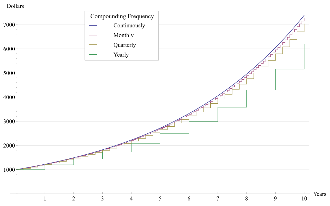
To compare apples to apples, we must find the Effective Annual Rate (EAR). The EAR represents the true return earned or interest paid on an investment or loan after accounting for the compounding frequency.
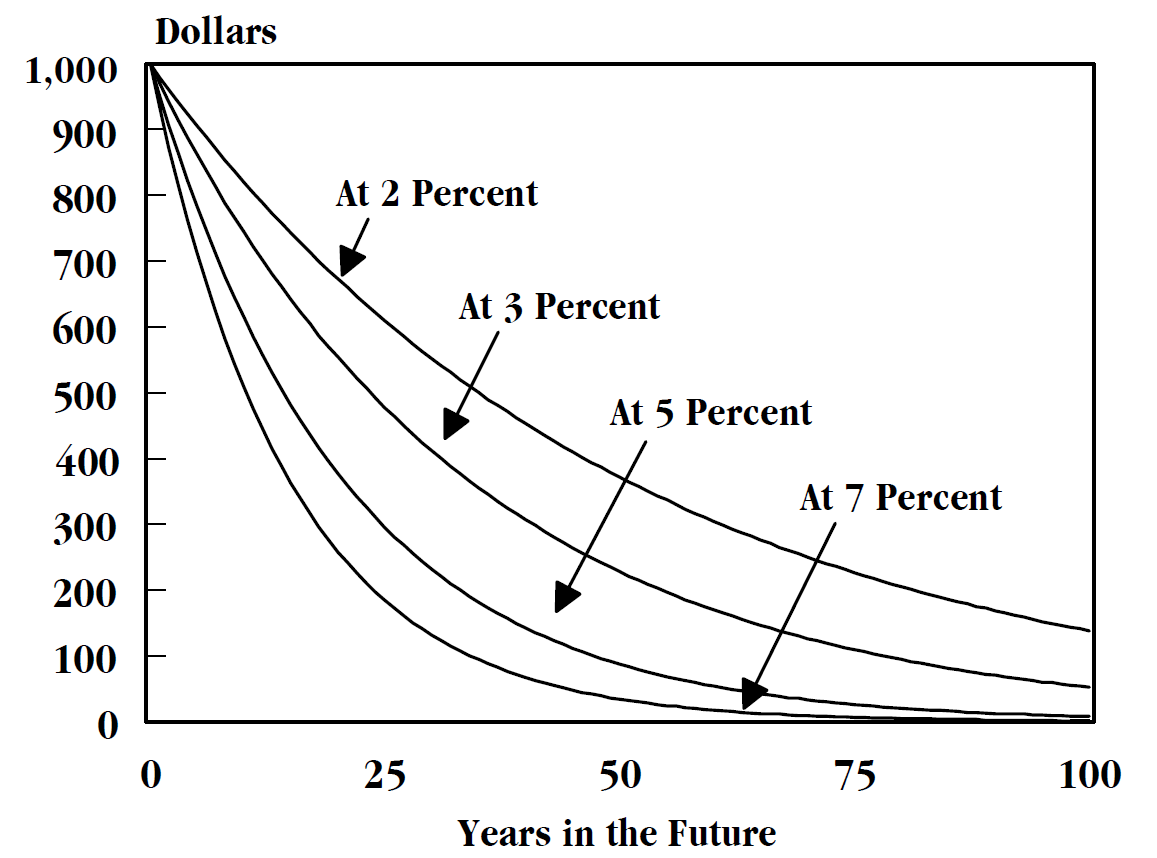
Just as compounding frequency acts as an accelerator for Future Value, the discount rate acts as gravity on Present Value. Increasing the discount rate applied to an analysis decreases the present value of a future sum of money. If you demand a higher rate of return (a higher discount rate), you are willing to pay less today for a future dollar.
In reality, clients rarely invest a single lump sum and walk away. They save monthly, or they draw down quarterly. We must categorize these recurring streams of cash to model them correctly.
Ordinary Annuities vs. Annuities Due
An annuity is simply a predictable stream of cash flows. The timing of those flows changes the math entirely.
- An ordinary annuity consists of a series of equal payments made at the end of each consecutive period.
- An annuity due consists of a series of equal payments made at the beginning of each consecutive period.
Why does this matter? Because of compounding. If a client deposits money at the beginning of the year, that capital has the entire year to grow. Therefore, an annuity due will always produce a higher present value than an ordinary annuity with an identical payment amount and interest rate.
| Characteristic | Ordinary Annuity | Annuity Due | Common CFP® Applications |
|---|---|---|---|
| Timing of Cash Flow | End of period | Beginning of period | |
| Compounding Periods | n−1 periods of growth | n periods of growth | |
| Mathematical Weight | Lower PV and FV | Higher PV and FV | |
| Real-World Examples | Debt payments, Bond coupons | Rent, Tuition, Retirement income |
Irregular and Infinite Flows
Life does not always fit neatly into fixed annuities. Uneven cash flow analysis is utilized when an investment produces periodic cash flows that vary in amount over time. Valuing a business or analyzing real estate requires discounting each unique cash flow back to the present individually.
What if the cash flow never stops? A perpetuity is a specialized type of annuity that pays a continuous and equal cash flow indefinitely into the future. Preferred stocks are classic examples.
Present Value of a Perpetuity The present value of a perpetuity is calculated by dividing the periodic payment amount by the applicable discount rate. PV=RatePayment
This elegantly simple equation is incredibly powerful. It forms the foundation of the capitalization of earnings method, which determines the present value of an infinite stream of income by dividing the expected annual income by the capitalization rate. It tells a buyer exactly what a stream of perpetual income is worth today.
If we project a client’s wealth using nominal rates, we are giving them a dangerous illusion. Wealth is not measured in dollars; it is measured in purchasing power.
A real rate of return is the annual percentage return realized on an investment adjusted for changes in prices due to inflation. You must strip away the inflationary "fat" to find the "muscle" of actual wealth creation.
Inflation-Adjusted Return Formula The inflation-adjusted return formula requires dividing one plus the nominal rate by one plus the inflation rate before subtracting one from the result. Real Rate=[1+Inflation Rate1+Nominal Rate]−1
When funding long-term goals, planners utilize serial payments—a series of payments that systematically increase each period to exactly match the assumed rate of inflation. This ensures the client's purchasing power remains constant over time.
For rapid, back-of-the-napkin estimates of purchasing power or growth without a calculator, planners rely on a classic heuristic: The Rule of 72. This estimates the number of years required to double an investment by dividing the number 72 by the annual interest rate. If inflation is 3%, prices will double in 24 years (72/3). If an investment earns 8%, it doubles in 9 years (72/8).
When evaluating investments, financial planners act as corporate CFOs for their clients' households. We must distinguish between projects that destroy wealth and those that create it. We do this using Net Present Value and the Internal Rate of Return.
Net Present Value (NPV) calculates the difference between the present value of cash inflows and the present value of cash outflows over a specific time horizon. It measures absolute wealth creation in today's dollars.
- The NPV Rule: An investment is considered acceptable under the Net Present Value rule if the calculated Net Present Value is greater than zero. If NPV is positive, the investment has exceeded the required rate of return and mathematically increased the client's net worth.
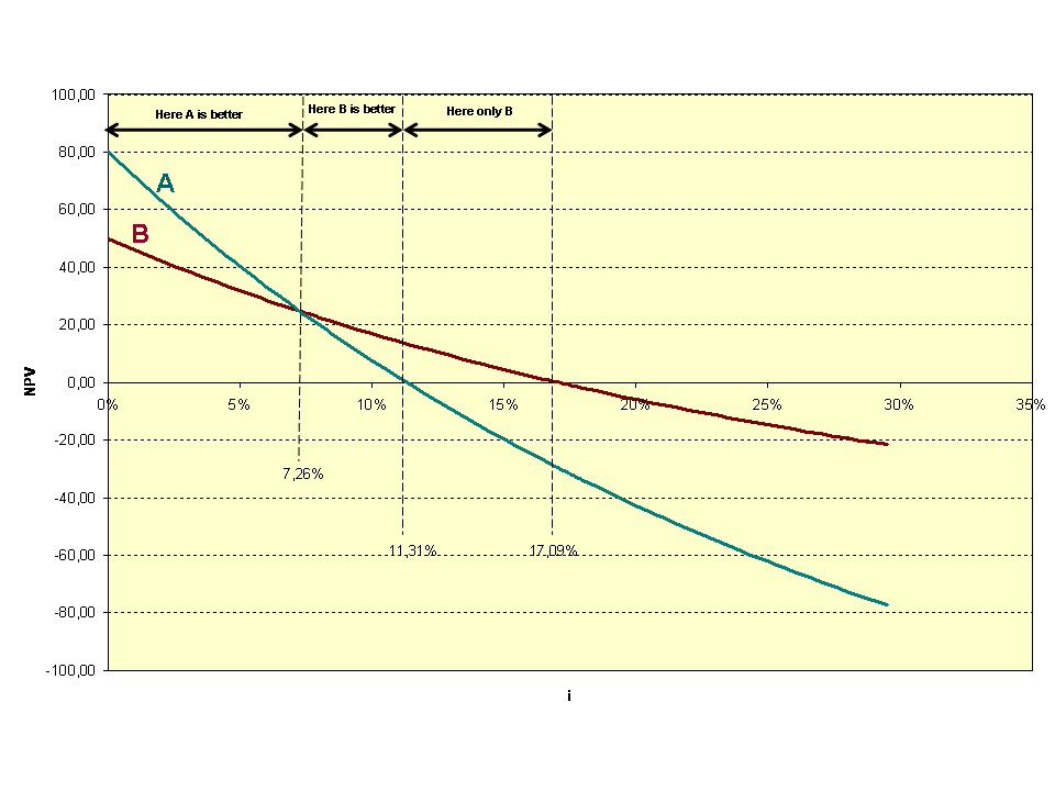
The Internal Rate of Return (IRR) is the exact discount rate that results in a Net Present Value of exactly zero. It represents the annualized yield of an investment.
- The IRR Rule: An investment is considered acceptable under the Internal Rate of Return rule if the calculated Internal Rate of Return exceeds the investor's required rate of return.
The Superiority of NPV and the Reinvestment Trap
While clients love IRR because a percentage is easy to digest (e.g., "This real estate syndication yields 15%"), the IRR metric harbors a dangerous mathematical flaw.
The standard Internal Rate of Return formula inherently assumes that all intermediate cash flows from a project are reinvested at the Internal Rate of Return itself.
If an exotic investment boasts a 25% IRR, the math blindly assumes the client takes every dividend and instantly reinvests it somewhere else at a guaranteed 25%. In reality, that cash likely sits in a money market account earning 4%.
For this reason, the Net Present Value method is mathematically superior to the Internal Rate of Return method when evaluating mutually exclusive investment projects. NPV correctly assumes cash flows are reinvested at the firm's (or household's) conservative cost of capital.
To fix IRR's flaw, analysts use the Modified Internal Rate of Return (MIRR). MIRR assumes that intermediate positive cash flows are reinvested at the firm's cost of capital or another specified external reinvestment rate, providing a significantly more accurate picture of reality.
The CFP® exam is not a math test; it is a scenario analysis test. You must know exactly which TVM assumptions apply to specific life events.
Debt and Mortgages
Debt is a stream of cash flows directed away from the client. Mortgage payments and standard consumer loan amortizations are mathematically calculated using ordinary annuity assumptions. You occupy the house for the month, and you pay for it at the end of the month.
Amortization schedules mathematically separate periodic loan payments into their respective principal repayment and interest expense components. Because the outstanding principal is highest on day one, in the early years of a fully amortizing loan, the vast majority of the periodic payment is applied toward the interest expense rather than the principal balance. As the principal slowly decreases, less interest accrues, and a larger fraction of the fixed payment attacks the principal.
Occasionally, loans are not fully amortizing. They may feature a balloon payment, which is an unusually large lump sum payment scheduled at the end of a loan term to satisfy the remaining principal balance.
Education Funding
Universities do not let students sit through a semester and bill them at the end. Education tuition payments are modeled as occurring at the beginning of each academic period as an annuity due. Using ordinary annuity mode for an education goal will mathematically under-fund the client's needs.
Retirement Income and Distribution Strategies
Similarly, you cannot buy groceries in retirement by promising to pay the supermarket at the end of the month. Retirement income calculations typically assume distributions occur at the beginning of each period as an annuity due.
When calculating the total capital required to fund a retirement, planners choose from three distinct philosophical approaches:
- The capital depletion approach to retirement planning assumes the retirement account balance will reach exactly zero at the end of the life expectancy period. This requires the least amount of savings today but leaves no inheritance and risks outliving the money if the client exceeds life expectancy.
- The capital preservation approach assumes the original principal balance will remain fully intact at the end of the life expectancy period. The client essentially lives only on the real growth.
- The purchasing power preservation approach assumes the original principal balance will retain its inflation-adjusted purchasing power at the end of the life expectancy period. This is the most conservative and requires the largest nest egg today, guaranteeing a robust legacy.

A brilliant strategy is useless if it is entered into the calculator incorrectly. The financial calculator (whether the HP-12C or TI BA II Plus) acts as a mechanical ledger, and it demands perfect accounting of cash direction.
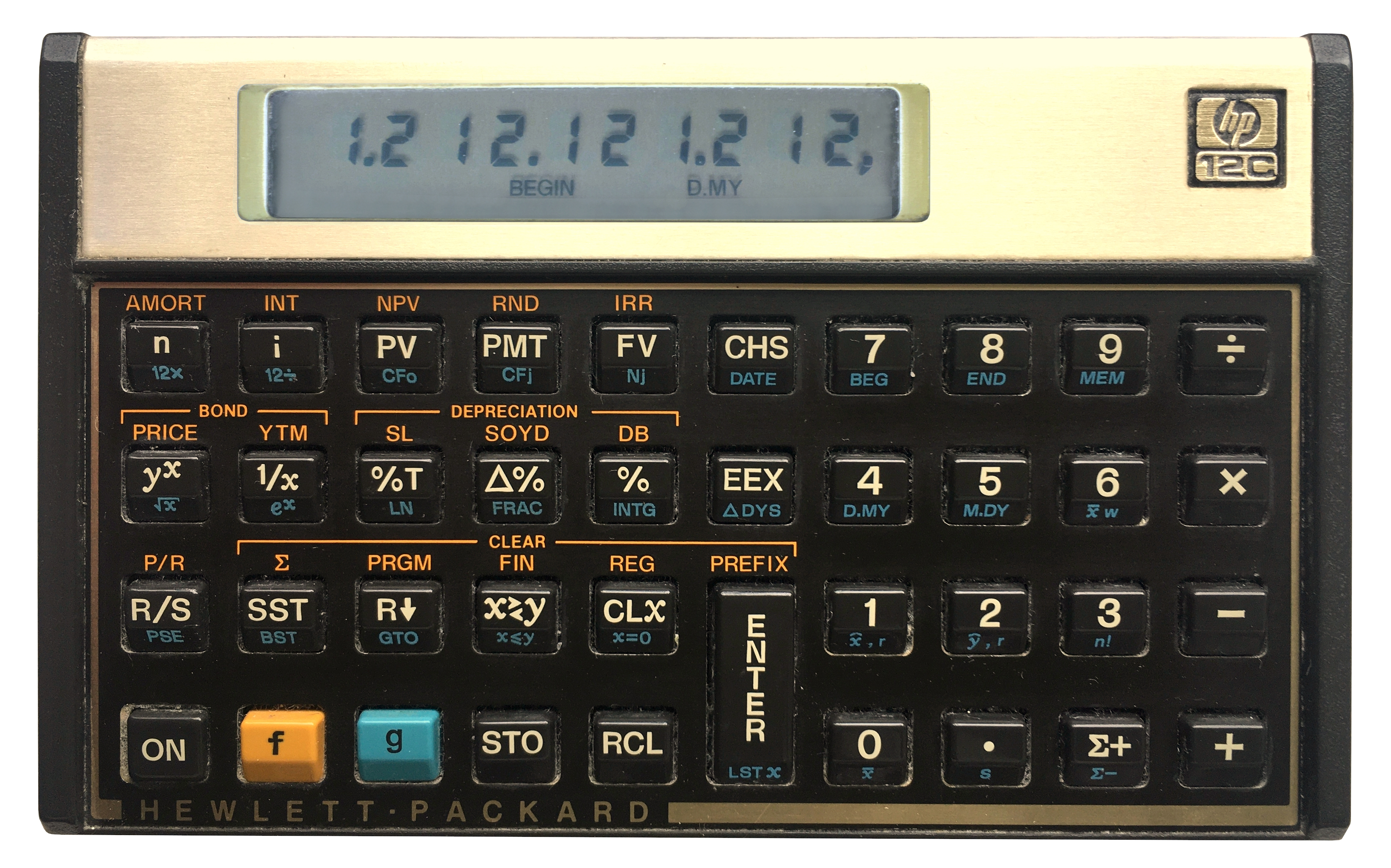
In standard financial calculator usage, the Present Value cash flow must be entered with an opposite mathematical sign to the Future Value cash flow to compute correctly.
Think of the calculator as tracking a wallet. If you deposit $10,000 into an investment today (Present Value), that money has left your wallet. It is entered as a negative number (-10,000). When the investment matures in ten years (Future Value), the money returns to your wallet. The calculator will output a positive number. If you enter both as positive, the calculator will return an error, because it cannot comprehend a scenario where you receive money today and receive money tomorrow without ever having made an initial outlay.
Understanding the mechanics of time, interest, inflation, and cash flow direction is the bedrock of financial planning. When you master the Time Value of Money, you are no longer just guessing at a client's future—you are engineering it.