Retirement needs analysis
Consider the fundamental physics of a human lifetime's economic output. For roughly four decades, an individual converts their labor into a kinetic stream of income, relying on its continuous flow to fund their standard of living. Upon retirement, this dynamic engine is intentionally shut down. To survive the remainder of their life, the individual must have amassed a reservoir of stored potential energy—financial capital—large enough to sustain a steady outward flow until they die. The mathematical modeling of this transition is the retirement capital needs analysis.
For the comprehensive financial planner, this analysis is not merely a rote calculation; it is the structural engineering of a client's future. If your math is flawed, the reservoir runs dry. To prevent this, we must precisely quantify the demand (how much income the client will need), account for the friction of time and inflation, and determine exactly how much capital is required to safely supply that demand.
Before calculating a target portfolio size, you must isolate the exact dollar amount the client will need to spend. We achieve this through two primary modeling approaches.
The Wage Replacement Ratio Method
The Wage Replacement Ratio method is a macro-level approach that estimates retirement income needs as a fixed percentage of preretirement gross income. It assumes a client's standard of living is inextricably tied to their preretirement salary, but acknowledges that not every dollar earned today needs to be replaced tomorrow.
A widely accepted standard baseline for the Wage Replacement Ratio is 70 to 80 percent of preretirement income. But where does this percentage come from? It relies on the Top-Down approach, which applies standard percentage reductions to preretirement income to account for expenses that simply vanish when labor ceases.
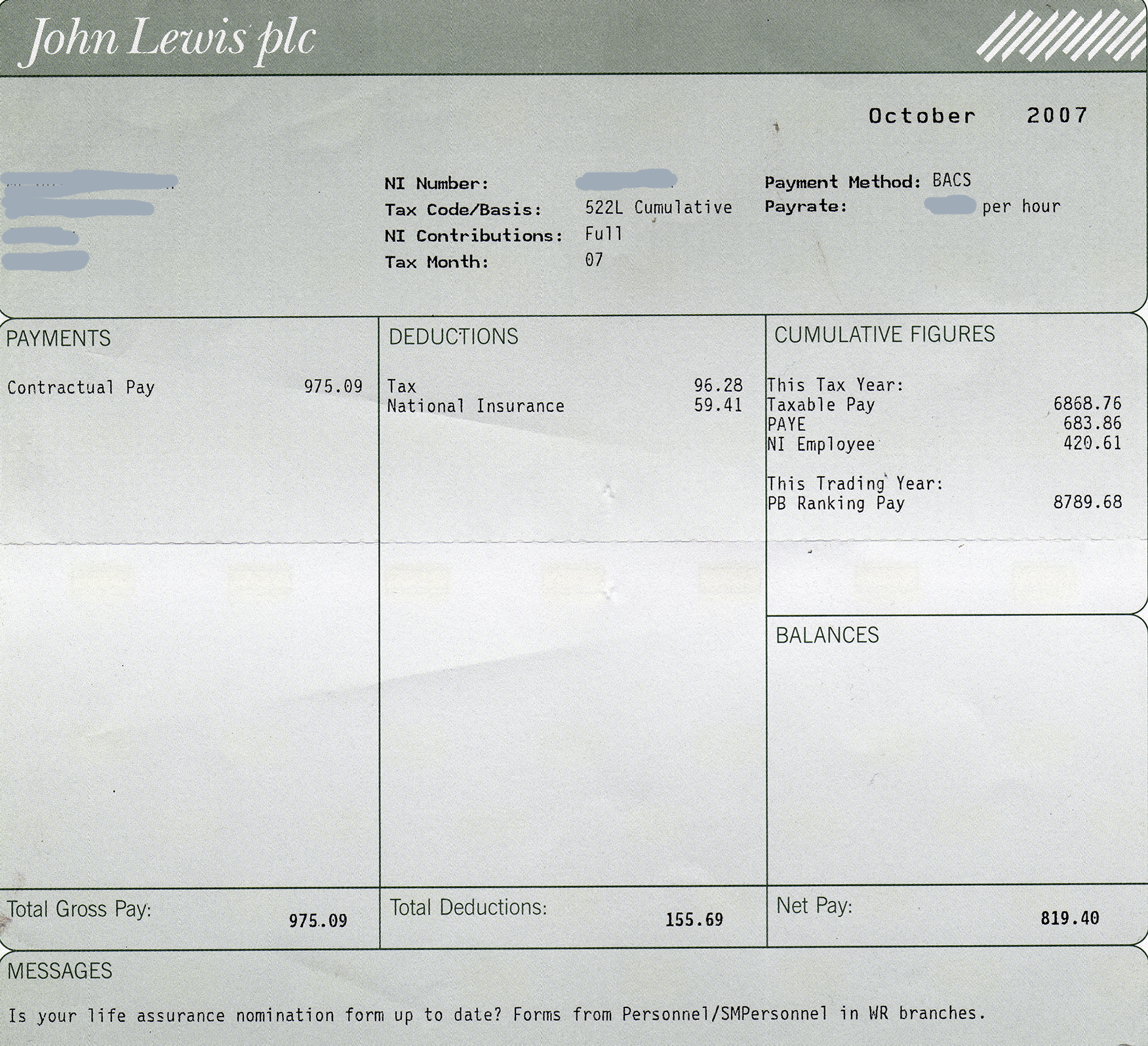
If you want to calculate a highly precise Wage Replacement Ratio rather than relying on standard rules of thumb, you look at the client's pay stub and subtract the specific cash flows that will end at retirement. For instance, payroll taxes are subtracted from preretirement income because FICA taxes only apply to earned wages. Similarly, preretirement savings contributions are subtracted from preretirement income because the client is transitioning from the accumulation phase to the distribution phase; they no longer need to save for the very event they are currently experiencing.
The Bottom-Up Approach
If the Wage Replacement Ratio is a macro-estimate, the Bottom-Up approach is a micro-level reconciliation. Instead of reducing current income, the Bottom-Up approach calculates retirement income needs by aggregating specific anticipated individual living expenses.
When you sit with a client utilizing this method, you are building a new budget from scratch. Work-related expenses like commuting costs are omitted from projected expenses, as the client is no longer driving to the office or paying for dry cleaning. Conversely, new structural costs appear. Most notably, Medicare premiums are added as a new anticipated expense when projecting retirement needs using the Bottom-Up approach.
Whether using the Top-Down or Bottom-Up method, the raw expense number is just the beginning. A comprehensive capital needs calculation must inflate current living expenses to their future value at the expected retirement date. A $100,000 lifestyle today will cost significantly more twenty years from now.
Isolating the Retirement Income Shortfall
Once you have the total projected, inflation-adjusted retirement expenses, you must account for external safety nets. Expected Social Security benefits are subtracted from total projected retirement expenses to determine the retirement income shortfall.
The Retirement Income Shortfall is the specific dollar amount of retirement expenses that must be funded by personal investment capital.
This shortfall is the critical output of your expense modeling. It is the exact gap your investment portfolio must bridge.
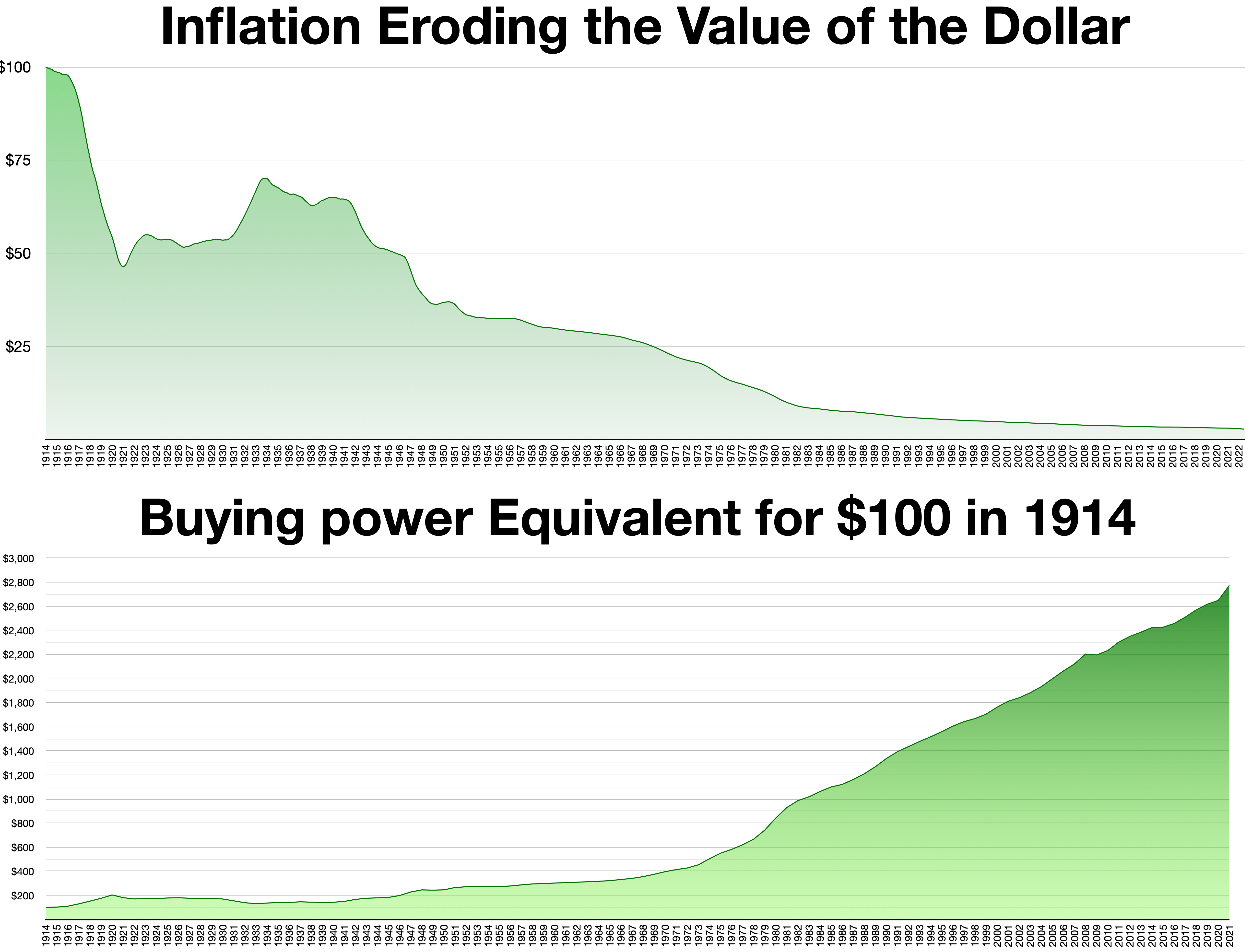
In financial physics, inflation is entropy. It constantly erodes the purchasing power of the client's cash flow. When modeling retirement withdrawals over several decades, we must rely on serial payments. Serial payments in retirement distributions are payment amounts that increase periodically by the inflation rate. Because they scale upward synchronously with inflation, serial payments maintain constant purchasing power for the retiree throughout the distribution period.
To model these serial payments accurately, we cannot simply use a standard nominal interest rate to discount future cash flows. The inflation-adjusted rate of return must be used as the discount rate when evaluating future retirement cash flows that grow with inflation.
Formula: The inflation-adjusted rate of return is calculated as: (1+inflation rate1+nominal return)−1
Notice the relationship inherent in this denominator. An increase in the anticipated inflation rate decreases the calculated inflation-adjusted rate of return. When the real rate of return shrinks, the investment portfolio is doing less "work" to sustain the withdrawals. Consequently, a lower inflation-adjusted rate of return increases the present value of the required retirement capital. The less your money grows in real terms, the more money you must supply upfront.
The Annuity Due Assumption
When calculating the present value of these serial payments, timing is paramount. Retirement withdrawal calculations typically utilize an annuity due assumption rather than an ordinary annuity assumption. An annuity due assumption signifies that retirement withdrawals occur at the absolute beginning of each payment period.
Think of a retiree's actual life: they need cash on the first day of the month to pay their mortgage and buy groceries. They do not wait until the end of the month to consume. Setting your financial calculator to "BEG" mode accurately reflects this reality and slightly increases the required capital compared to an ordinary annuity.
We now arrive at the core calculation. The first step of a retirement capital needs analysis calculates the present value of the retirement income shortfall at the exact retirement date.
The calculated present value of the retirement income shortfall represents the target capital balance needed to successfully retire.
How you determine this target balance depends entirely on what the client wants left over when they die. We model this using three distinct methods:
| Method | Definition | Outcome at Life Expectancy |
|---|---|---|
| Capital Depletion Method | Calculates the retirement capital needed to exhaust all funds exactly at the end of the projected life expectancy. | Zero dollars remaining. |
| Capital Preservation Method | Determines the required retirement capital to maintain the original nominal principal balance at death. | Original nominal starting amount remains. |
| Purchasing Power Preservation Method | Calculates the required retirement capital to maintain the inflation-adjusted principal balance at death. | Original principal, adjusted upward for cumulative inflation, remains. |
The capital depletion method is the most highly tested baseline approach. Because it assumes the portfolio drops to zero on the final day of the projection, it requires the least amount of starting capital. In academic planning, the capital depletion method is also known as the pure annuity method, conceptually mirroring the payout structure of a single-premium immediate life annuity.
Conversely, the purchasing power preservation method requires the largest initial retirement capital balance among the three primary capital needs methods. By demanding that the portfolio not only spin off cash to live on but also grow its principal base perfectly in tandem with inflation to leave a massive legacy, it places immense pressure on the starting balance.
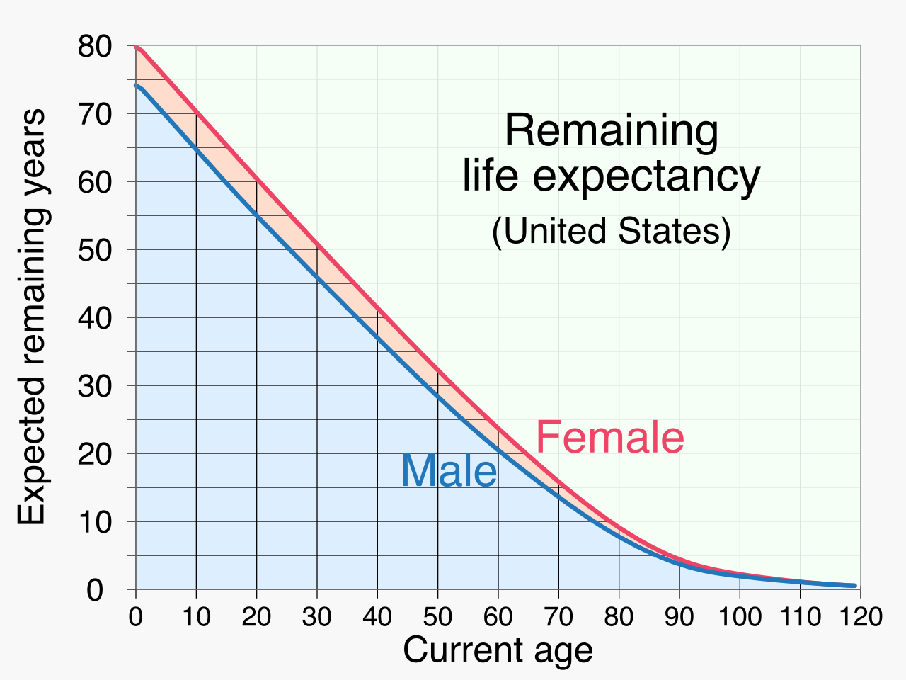
Modeling for Longevity Risk
Regardless of the method chosen, the target capital balance is fundamentally sensitive to the assumed timeframe. Increasing the projected life expectancy in a retirement model increases the total capital required at the retirement start date.
If you miscalculate a client's life expectancy, you expose them to longevity risk, which is the danger of a retiree outliving their accumulated investment capital. In the academic literature, this catastrophic scenario has a precise name: superannuation is a formal financial planning term describing the risk of a person outliving their money. Overestimating investment returns or underestimating life expectancy are the primary drivers of superannuation.
Once the target capital balance at retirement is established, the final mathematical requirement shifts to the client's current reality. The second step of a retirement capital needs analysis calculates the required periodic savings needed during the working years to reach the target retirement capital. This is a standard future value accumulation problem, establishing the annual or monthly savings goal required today to fill the reservoir by tomorrow.
The 4 Percent Rule
While comprehensive modeling utilizes exact discounting and present-value calculations, planners frequently employ heuristics for quick scenario testing. The most famous is the 4 percent rule, which suggests a safe initial retirement withdrawal rate of 4 percent of the starting portfolio value.
The elegance of this rule lies in its mechanics regarding inflation. The 4 percent rule assumes annual withdrawal amounts are increased each subsequent year to exactly match inflation, functioning perfectly as a serial payment. If a client retires with a $1,000,000 portfolio, they withdraw $40,000 in year one. If inflation is 3%, year two's withdrawal is $41,200. The rule dictates that historically, a diversified portfolio subjected to this exact withdrawal pattern is highly unlikely to face superannuation over a 30-year timeframe.
For the CFP® professional, understanding these underlying dynamics—from the granular calculation of a Wage Replacement Ratio to the macroeconomic impacts of the inflation-adjusted discount rate—is what elevates you from a product salesperson to a true architect of financial independence.