Plan and Manage Finance: Allocations
Not sure you’re ready?
Take the ~3-minute readiness diagnostic and see where you stand.
In any complex system, whether a steam engine or an enterprise software deployment, energy must be precisely allocated, measured, and buffered against entropy. For the project manager, capital is that energy. Managing project finance is not merely an accounting exercise of balancing ledgers; it is the physical manifestation of strategy, risk, and delivery mapped across time. Every dollar allocated represents a quantifiable unit of effort, and every financial reserve acts as a necessary shock absorber against the inherent uncertainty of execution. Understanding how to estimate these requirements, structure the baseline, quantify the buffers, and track the burn of capital is what separates a naive schedule from a mathematically robust delivery framework.
Before we can manage project capital, we must accurately forecast our requirements. The methods we choose depend heavily on the maturity of the project's scope and the project life cycle—whether predictive, agile, or hybrid.
To calculate foundational costs, project managers utilize several distinct estimating techniques:
- Analogous estimating uses historical data from similar past projects to estimate current project costs. If an infrastructure upgrade cost $500,000 last year, analogous estimating uses that figure as a top-down starting point. It is rapid but relies entirely on the premise that the past is a strictly accurate prologue.
- Parametric estimating uses statistical relationships between historical data and project variables to calculate cost estimates. If laying fiber optic cable costs $15 per linear foot, and the project requires 10,000 feet, the parametric estimate is inherently mathematical and scalable.
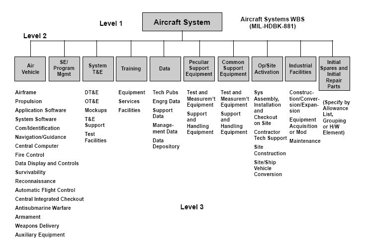
- Bottom-up estimating aggregates individual work package costs to determine the total project cost. By estimating every granular task in the Work Breakdown Structure (WBS) and rolling those figures upward, you achieve the highest fidelity of accuracy, albeit at the expense of significant time and effort.
Conversely, agile projects frequently use lightweight estimation methods like relative sizing to forecast financial needs. Rather than fixating on absolute dollar amounts for unknown granular tasks, agile practitioners estimate the relative effort (such as story points) to forecast how much work a team can accomplish over time. Because agile assumes scope will evolve, agile projects often fund continuous value streams or cross-functional teams rather than individual project phases. You are effectively funding a predictable engine of execution—a dedicated team over a set duration—rather than a rigid list of predetermined deliverables.
A pure aggregation of task estimates assumes a frictionless world. Reality, however, is fraught with entropy. To construct a viable budget, we must translate physical project risks into financial allocations. We classify these buffers into two distinct categories: Contingency Reserves and Management Reserves.
Sizing the Buffer: EMV and Monte Carlo
To justify a financial buffer, we cannot rely on intuition; we must quantify the risk.
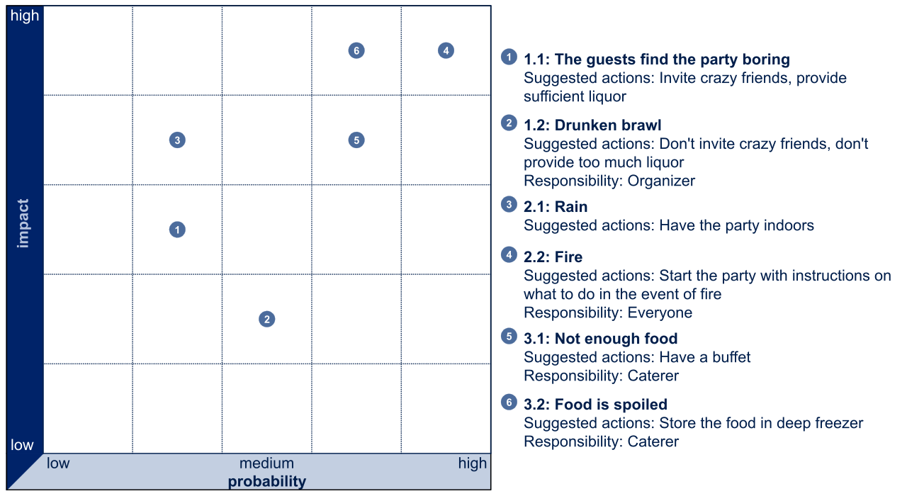
Expected Monetary Value (EMV) calculates average risk cost by multiplying the probability of a risk by the financial impact. If a supply chain delay has a 40% probability of occurring and would cost the project $50,000 in penalties, the EMV for that specific risk is $20,000. You aggregate these EMVs to help establish a baseline risk budget.
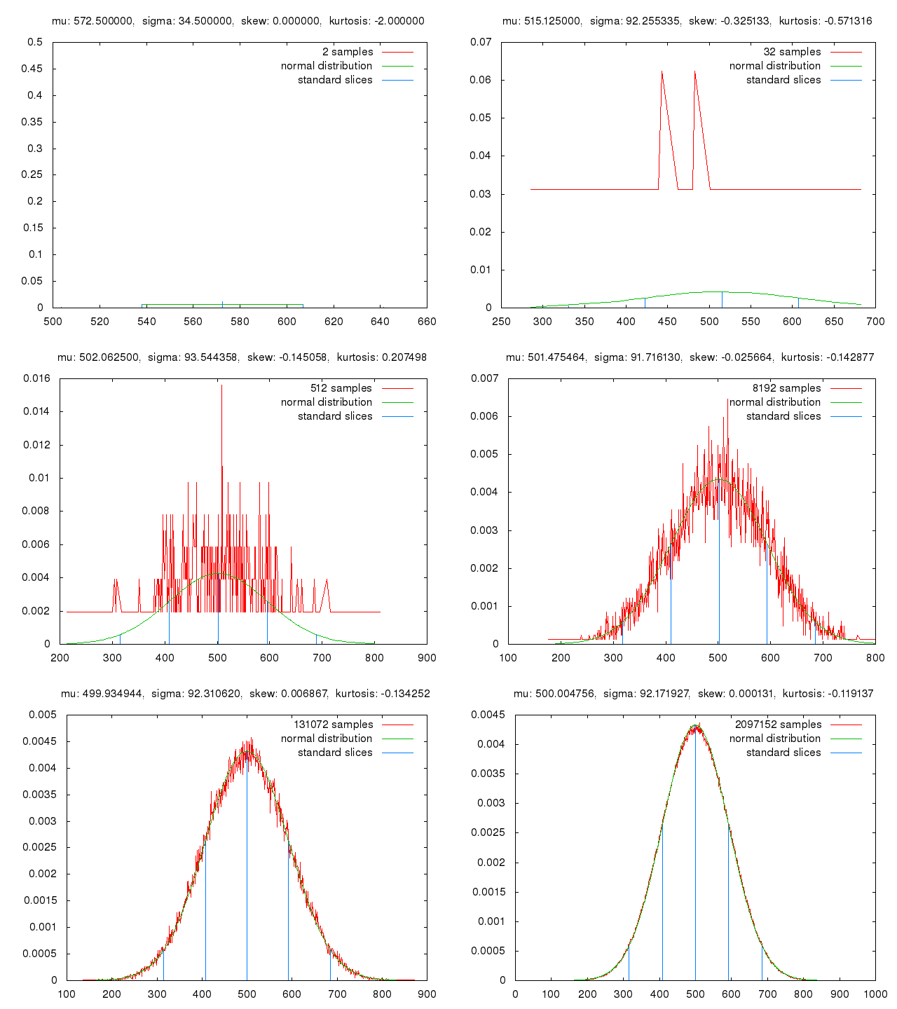
However, project risks do not occur in a vacuum; they interact. A Monte Carlo simulation models the probability of different project cost outcomes based on identified risk variables. By running thousands of automated, randomized simulations of the project schedule and budget, the Monte Carlo method provides a probabilistic curve—telling management, for example, that there is an 80% confidence level the project will finish at or below $1.2 million.
Contingency vs. Management Reserves
Once quantified, funds are placed into distinct operational buckets based on the nature of the risk.
Contingency reserves provide financial allocations to cover "known-unknown" risks identified in the risk register. These are the risks we foresaw and quantified using EMV or Monte Carlo. Because these are planned buffers, the project manager has the authority to use contingency reserves without submitting a formal change request.
Management reserves, in stark contrast, provide financial allocations to cover "unknown-unknown" risks not previously identified by the project team. This is the organizational shock absorber for emergent, unforeseeable disasters—a sudden global pandemic or a previously unknown geological fault line under a construction site. Because these funds are held outside the project manager's baseline control, the use of management reserves requires an approved formal change request.
Understanding how these reserves nest within the project's financial structure is a fundamental requirement of project finance:
The Cost Baseline represents the approved version of the time-phased project budget. The cost baseline excludes management reserves, meaning it consists solely of your aggregated task estimates plus your contingency reserves.
The Total Project Budget, however, includes both the cost baseline and management reserves.
If an unknown-unknown risk occurs and a change request is approved to utilize those emergency funds, a structural shift happens: reallocating management reserve into the cost baseline increases the overall authorized project cost baseline.
Establishing a budget does not mean the organization hands the project manager a vault of cash on day one. Enterprise cash flow is tightly orchestrated. Funding limit reconciliation regulates the expenditure of project funds according to organizational funding constraints. If your baseline requires $100,000 in Q1 but the corporate treasury only releases $75,000 per quarter, you must reconcile your schedule—delaying certain activities to ensure the project's burn does not exceed the organization's available liquidity.
Tracking this flow of capital differs wildly by methodology. Predictive projects establish a detailed cost baseline upfront for tracking financial performance throughout the life cycle. Every dollar is mapped to a point in time.
By contrast, agile teams track spend dynamically through sprint-based burn rates. A burn rate calculates how fast an agile team consumes the project budget over a specific time period (e.g., spending $40,000 per two-week sprint). If the team's burn rate remains constant, forecasting financial exhaustion becomes a straightforward exercise in dividing the remaining budget by the burn rate.
In predictive and hybrid environments, tracking money spent against time passed is mathematically insufficient. If you have spent 50% of your budget halfway through the timeline, you might assume you are perfectly on track. But what if you have only completed 20% of the actual work?
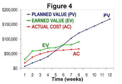
To solve this, we use Earned Value Management (EVM), a methodology that integrates scope, schedule, and cost. EVM relies on three foundational data points:
- Planned Value (PV) defines the authorized budget assigned to scheduled project work. (What did you plan to spend by today?)
- Earned Value (EV) measures the amount of work performed expressed in terms of the budget authorized for that specific work. (What is the budgetary value of the physical work you actually finished?)
- Actual Cost (AC) represents the realized cost incurred for the work performed on a schedule activity. (What did you actually pay out of pocket to do it?)
Calculating Variances and Indices
With PV, EV, and AC, we can calculate our absolute variances and our efficiency indices.
Cost Variance (CV) determines budget deficits or surpluses by subtracting Actual Cost from Earned Value (CV = EV - AC).
- A negative Cost Variance indicates that the project is currently over budget. You paid more than the physical work was worth.
- Conversely, a positive Cost Variance indicates that the project is currently under budget.
To understand our efficiency as a ratio, we use the Cost Performance Index (CPI). The Cost Performance Index measures cost efficiency by dividing Earned Value by Actual Cost (CPI = EV / AC).
- A Cost Performance Index below 1.0 indicates a cost overrun for the work completed. (e.g., a CPI of 0.80 means you are only getting 80 cents of value for every dollar spent).
- A Cost Performance Index above 1.0 indicates a cost underrun for the work completed.
| Metric | Formula | Interpretation | Meaning |
|---|---|---|---|
| Cost Variance (CV) | EV - AC | Negative | Over budget |
| Positive | Under budget | ||
| Cost Performance Index (CPI) | EV / AC | < 1.0 | Cost overrun (inefficient) |
| > 1.0 | Cost underrun (highly efficient) |
Historical metrics only tell us where we are. The project manager's primary duty is to look forward, utilizing EVM data to forecast future financial states.
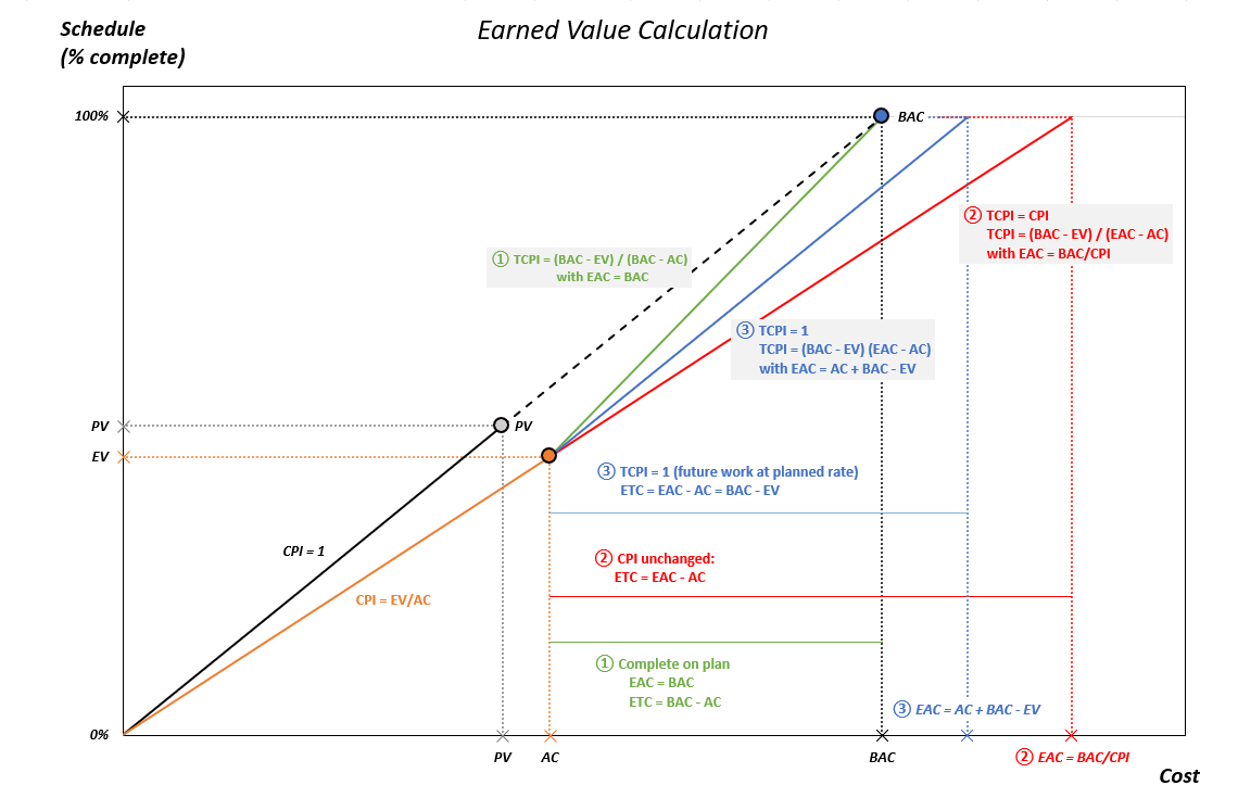
- Estimate at Completion (EAC) projects the total expected cost of the project based on current performance data. If your initial baseline was $100,000 but your CPI is persistently 0.80, your EAC will project a final cost significantly higher than your original plan.
- Estimate to Complete (ETC) projects the expected cost required to finish all remaining project work. It is the financial distance from today to the finish line.
- Variance at Completion (VAC) projects the expected budget deficit or surplus at the end of the project (VAC = Budget at Completion - EAC).
When a project goes off track, management often sets a strict financial ceiling to finish the work. The To-Complete Performance Index (TCPI) calculates the cost performance required to meet a specified management financial goal. If you have squandered budget early, your TCPI will rise above 1.0, meaning your team must work at an artificially high rate of cost efficiency for the remainder of the project just to break even.
Financial allocation is not a "set and forget" exercise. Throughout the execution phase, the risk landscape naturally evolves. Risks expire, and new threats emerge. Consequently, a project manager conducts reserve analysis iteratively to adjust financial allocations as project risks expire. Reserve analysis compares the amount of remaining contingency reserve to the severity of remaining project risks. If a scheduled hurricane season passes without incident, the risk profile decreases, and holding massive contingency reserves becomes capital inefficiency.
As the project successfully closes, financial reconciliation is finalized. Because contingency reserves are funded specifically for the risks within this distinct project, they do not belong to the project manager indefinitely. Upon completion, unused contingency reserves are typically returned to the organizational funding pool at project closure, allowing the enterprise to reinvest that capital into future value streams and continuous innovation.