Linear Equations and Inequalities
Not sure you’re ready?
Take the ~3-minute readiness diagnostic and see where you stand.
Picture a perfectly balanced physical scale in a laboratory. If a steel weight is placed on the left pan, a weight of identical mass must be placed on the right pan to preserve the equilibrium. Any action taken on one side must be perfectly mirrored on the other, or the system tips. At its core, an equation is a mathematical statement asserting that two expressions have the exact same value. The equal sign is not merely a prompt to calculate an answer; it is a rigid pivot point declaring perfect symmetry.
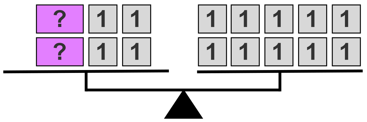
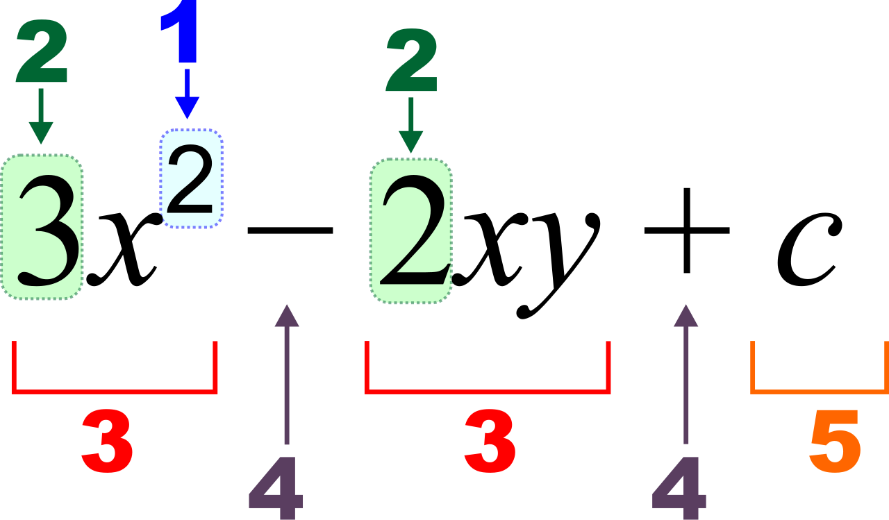
To understand the architecture of algebra, we begin with its most fundamental structure. A linear equation in one variable can be written in the form ax+b=c, where a, b, and c are real numbers and a is not equal to zero. Here, the variable acts as a placeholder for an unknown quantity—a hidden weight on our scale.
The objective of algebra is revelation. Solving an equation requires isolating the variable on one side of the equal sign using inverse operations. We systematically dismantle the mathematical scaffolding surrounding our unknown value by doing and undoing.
Nature relies on symmetry, and algebra provides the tools to reverse any operation:
- Addition and subtraction are inverse operations used to cancel out terms when solving an equation. If a constant has been added to our variable, we subtract that precise amount from both sides to maintain the scale's balance.
- Multiplication and division are inverse operations used to remove coefficients when solving an equation. If our variable is multiplied by a coefficient, dividing the entire equation by that coefficient unbinds the variable, leaving it completely isolated.
Real-world systems rarely present themselves in a neat, isolated format. They are often entangled in parentheses and scattered across the page. To solve a multistep equation, one must first simplify both sides by distributing and combining like terms before applying inverse operations. If you attempt to use inverse operations before organizing the equation, the mathematics becomes unnecessarily chaotic.
Breaking the Shells: The Distributive Property
When variables are trapped inside parentheses, we must unlock them. The distributive property states that a multiplied by the sum of b and c equals ab plus ac. Functionally, the distributive property is used to eliminate parentheses in an algebraic expression. By multiplying the outer factor across every inner term, we break open the expression, allowing the internal components to interact freely with the rest of the equation.
Sorting the Pieces: Combining Like Terms
Once the parentheses are cleared, the resulting expression may resemble a disorganized toolbox. We must sort the contents. Like terms are mathematical terms that contain the exact same variables raised to the exact same powers. The term 3x and the term 5x are like terms; they measure the exact same kind of theoretical object. However, 3x and 4y, or 2x and 5x2, are fundamentally different species. They cannot be fused.
Combining like terms simplifies an equation by adding or subtracting the coefficients of those corresponding terms. Just as three apples plus five apples yields eight apples, 3x+5x yields 8x. We condense the chaos into a streamlined form before ever moving a term across the equal sign.
When isolating a variable, we typically arrive at a distinct destination, such as x=4. A linear equation with exactly one solution has a single numerical value that makes the equation true. But what happens when the variables completely vanish during the solving process? The resulting arithmetic determines the fabric of the solution space.
The Contradiction: If simplifying the equation results in an absurdity—such as 3=5—the system is broken. A linear equation has no solution if simplifying the equation results in a mathematically false statement. There is no conceivable real number that can save a contradictory premise.
The Tautology: Consider the equation 2(x+3)=2x+6. If we distribute the left side, we get 2x+6=2x+6. Subtracting 2x from both sides leaves 6=6. This is an eternal mathematical truth. A linear equation has infinitely many solutions if simplifying the equation results in a mathematically true statement where both sides are identical. Any real number substituted into the variable will preserve the balance.
Not every system requires perfect balance; sometimes we are concerned with thresholds, limits, and capacities. An inequality is a mathematical statement comparing two expressions using less than, greater than, less than or equal to, or greater than or equal to symbols.
The mechanics of solving inequalities mirror those of equations. Solving a one-variable inequality uses the same sequence of inverse operations as solving a one-variable equation. You isolate the variable by distributing, combining, and applying inverse operations. However, the fabric of an inequality bends under certain arithmetic transformations.
Consider the true statement 3<5. What happens if we multiply both sides by −1? The numbers transform into −3 and −5. On the geometric number line, −3 sits to the right of −5, making it the larger value. The relationship has inverted: −3>−5. Multiplying by a negative number reflects our values across zero, acting like a mirror that flips the universe backwards.
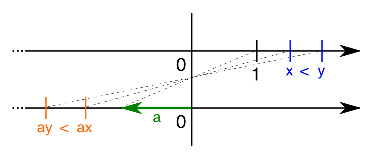
- Multiplying both sides of an inequality by a negative number reverses the direction of the inequality symbol.
- Dividing both sides of an inequality by a negative number reverses the direction of the inequality symbol.
Crucially, mere translation does not warp the space. Adding or subtracting a negative number from both sides of an inequality does not change the direction of the inequality symbol. Shifting the entire number line three units left does not alter the relative ordering of the points.

Because an inequality represents a continuous spectrum of valid solutions rather than a single point, we map these solutions visually.
The threshold itself determines our starting notation:
- On a number line graph, an open circle indicates that the specific boundary number is not included in the solution set. Consequently, the strictly less than and strictly greater than inequality symbols require an open circle when graphed on a number line. It is an asymptotic border; we can step infinitely close to the number, but we cannot stand on it.
- On a number line graph, a closed circle indicates that the specific boundary number is included in the solution set. Therefore, the less than or equal to and greater than or equal to inequality symbols require a closed circle when graphed on a number line. The boundary point is a valid solution.
Once the boundary is established, we shade the realm of truth:
- Graphing an inequality with a greater than symbol requires shading the number line to the right of the starting value, stretching toward positive infinity.
- Graphing an inequality with a less than symbol requires shading the number line to the left of the starting value, plunging toward negative infinity.
| Symbol | Meaning | Number Line Boundary | Shading Direction |
|---|---|---|---|
| > | Strictly greater than | Open Circle | Right |
| < | Strictly less than | Open Circle | Left |
| ≥ | Greater than or equal to | Closed Circle | Right |
| ≤ | Less than or equal to | Closed Circle | Left |
When we expand from one variable to two, we unlock the ability to model dynamic systems. A linear relationship represents a constant rate of change between an independent variable and a dependent variable. For every distinct step forward in our independent input (x), our dependent output (y) marches upward or downward by a strictly predictable, unchanging amount.
Anatomy of a Real-World Model
When translated into an algebraic equation (such as y=mx+b), the components hold immense physical significance.
- In a linear equation representing a real-world scenario, the coefficient attached to the variable typically represents the constant rate of change. If an electrician charges $75 per hour, 75 is the coefficient driving the cost upward with every passing hour.
- In a linear equation representing a real-world scenario, the constant term typically represents the initial starting value. If the same electrician charges a flat $50 arrival fee before any work begins, the constant term is 50.
Equations serve as predictive engines. Substituting a specific value for the independent variable into a linear equation yields the exact corresponding value of the dependent variable. If we want to know the cost of a 4-hour electrical job, we substitute 4 into our independent variable, allowing the math to churn out the exact final bill.
Recognizing Linearity in Tables and Graphs
Data does not always arrive as a neat equation; often, we must extract the relationship from raw observations.
If given a matrix of data points, a table of values represents a linear relationship if the ratio of the change in the output variable to the change in the input variable remains constant throughout the table. This is the essence of slope (ΔxΔy). If the output jumps by 10 every time the input steps forward by 2, the ratio (5) must never waver. If it does, the relationship is nonlinear.
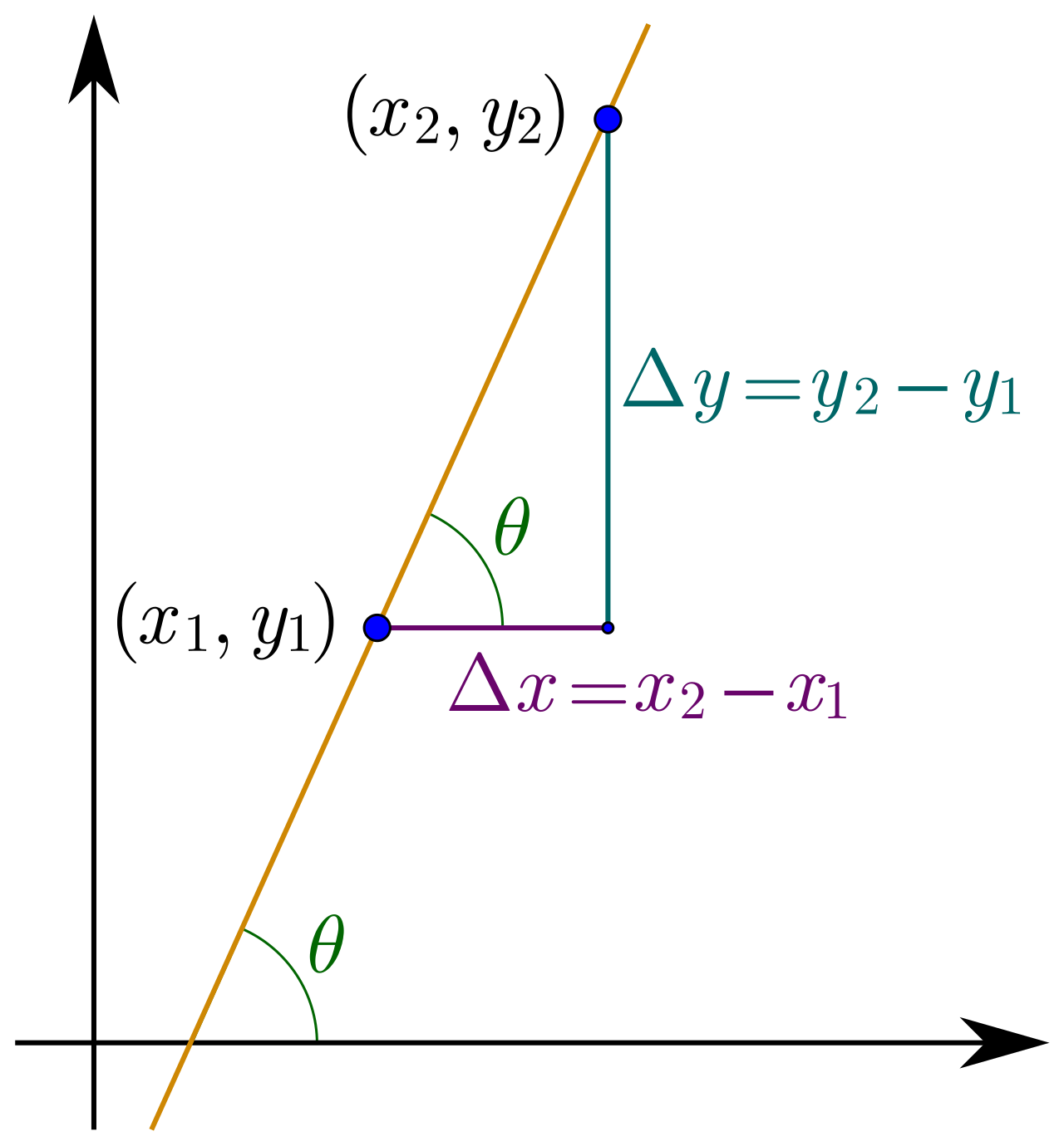
When we map this constant rhythm onto a two-dimensional Cartesian plane, geometry takes over. The graph of a linear relationship on a coordinate plane is always a perfectly straight line. There are no curves, parabolic arcs, or sudden fractures.
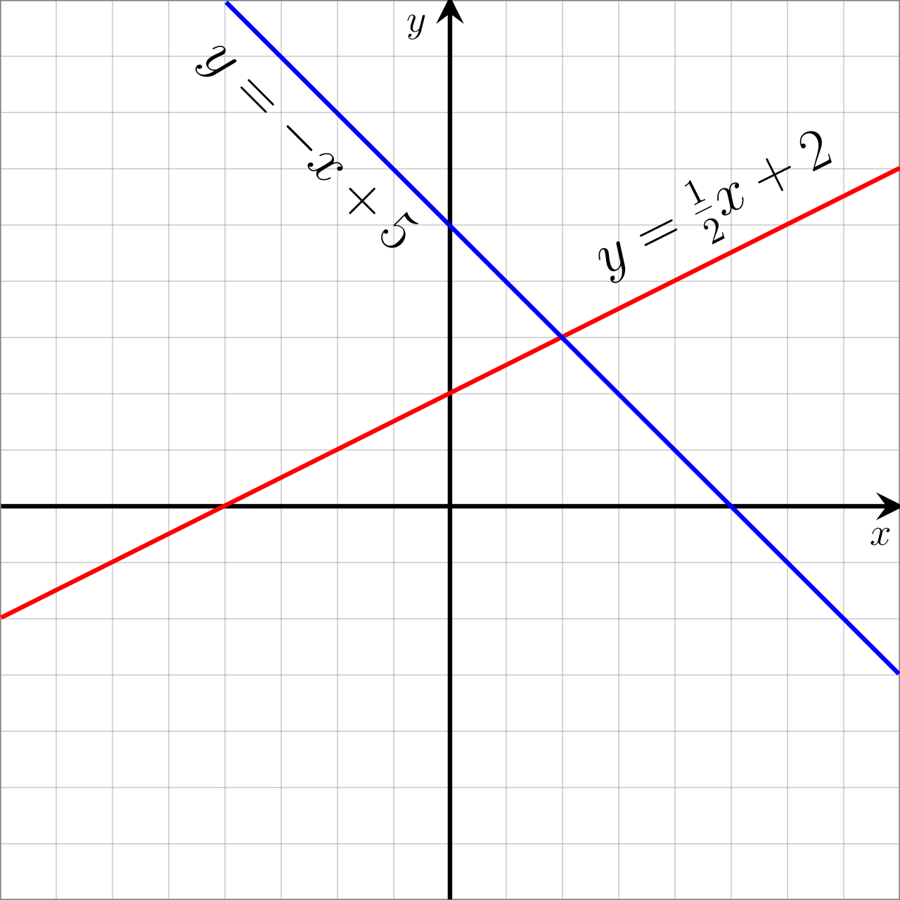
This line interacts with the foundational axes of our plane at critical junctions known as intercepts:
- The x-intercept of a linear graph is the coordinate point where the line crosses the horizontal x-axis. At this exact location, the dependent variable (y) is completely depleted, resting at zero.
- The y-intercept of a linear graph is the coordinate point where the line crosses the vertical y-axis.
The y-intercept is not merely a geometric curiosity; it is the genesis of our system. The y-intercept of a linear graph visually represents the initial value of the relationship when the independent variable is equal to zero. Looking back at our electrician, the graph of their fees will intersect the y-axis at exactly $50. Time has not yet begun (x=0), but the inherent baseline reality of the system (y=50) is already mathematically established.