Patterns and Functions
Not sure you’re ready?
Take the ~3-minute readiness diagnostic and see where you stand.
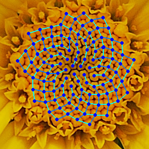
The universe does not operate on random chance; it runs on rhythms, structures, and deeply embedded rules. When a sunflower arranges its seeds, when a pendulum swings, or when an algorithm encrypts data, they all rely on the fundamental architecture of mathematics: the pattern. A mathematical pattern is an ordered set of numbers, shapes, or objects arranged according to a specific, predictable rule. To understand mathematics at its core is to learn how to recognize these rules, extend them into the unknown, and translate them into language that predicts the future. Every individual number, shape, or object within a mathematical pattern is called a term. By isolating how one term relates to the next, we transition from merely observing mathematics to actively controlling it.
To understand numerical patterns, we must first look at how they change from one term to the next. The nature of this change defines the family to which the pattern belongs.
Arithmetic Sequences: The Power of Constant Addition
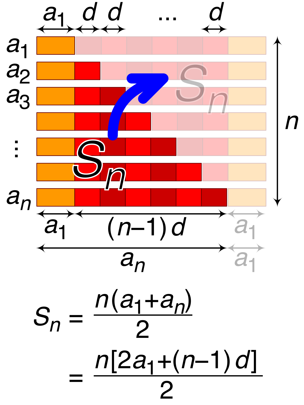
When a sequence grows or shrinks at a steady, unchanging rate, we are looking at the additive nature of arithmetic. An arithmetic sequence is a numerical pattern where each consecutive term is found by adding a constant value to the previous term. Because mathematics is beautifully symmetric, an arithmetic sequence can also be generated by subtracting a constant value from the previous term.
Definition: The constant value added or subtracted to find the next term in an arithmetic sequence is called the common difference.
Take the sequence 5,8,11,14,17. The common difference is +3. If we have the sequence 20,15,10,5,0, the common difference is −5. In both cases, the structural integrity of the pattern relies on an unbroken chain of identical steps.
Geometric Sequences: The Power of Multiplicative Scaling
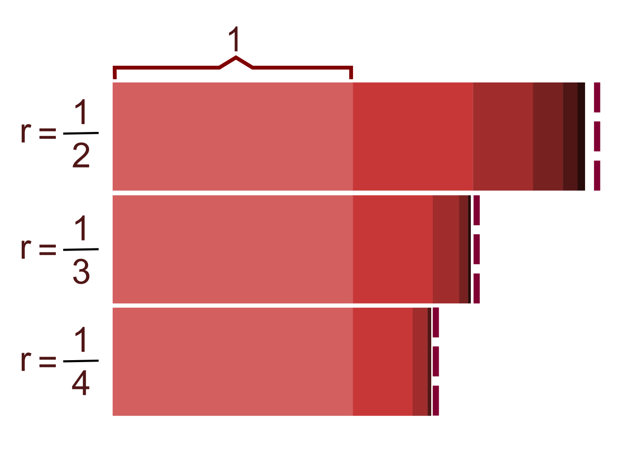
If arithmetic sequences represent climbing a staircase one step at a time, geometric sequences represent population growth, compounding interest, and exponential decay. A geometric sequence is a numerical pattern where each consecutive term is found by multiplying the previous term by a constant value. Conversely, a geometric sequence can also be generated by dividing the previous term by a constant value.
Definition: The constant value used to multiply or divide terms in a geometric sequence is called the common ratio.
Consider the sequence 2,6,18,54. The sequence scales rapidly because the common ratio is ×3. If we look at 64,32,16,8,4, the common ratio is ÷2 (or multiplying by 21). The behavior of geometric sequences is multiplicative, scaling up or shrinking down by a precise, repeated factor.
Before young students master the abstraction of numbers, they recognize structure through geometry and physical objects. Understanding shapes mathematically builds the visual-spatial reasoning necessary for algebra.
There are two primary ways shapes are utilized in pattern recognition:
- Repeating Shape Patterns: A repeating shape pattern consists of a core group of shapes that duplicates continuously in the exact same sequence. If you see a sequence arranged as Square, Triangle, Circle, Square, Triangle, Circle, the core group is the three shapes. Predicting the 10th or 100th shape in the pattern requires identifying this core and understanding its cycle.
- Growing Shape Patterns: Unlike a repeating cycle, a growing shape pattern is a sequence of shapes that increases or decreases in size or quantity according to a specific mathematical rule. Imagine a single square block. The next term is a 2×2 grid of blocks. The next is a 3×3 grid. The shapes are physically expanding in a way that directly correlates to an underlying numerical sequence.
Recognizing a pattern is only the first step; the ultimate goal is to formulate a rule that governs it. How we articulate that rule determines how far into the sequence we can efficiently calculate.
Recursive vs. Explicit Rules
Imagine you are analyzing the arithmetic sequence 4,7,10,13,16.
If someone asks you for the next term, you instinctively say 19. You know this because a recursive rule defines the next term in a sequence based entirely on the mathematical value of the immediately preceding term. The recursive rule here is simply "add 3 to the previous number." But what if someone asks you for the 1,000th term? Using a recursive rule would be incredibly tedious—you would have to find the 999th term first.
To bypass this, we look for a more powerful tool. An explicit rule calculates the value of any term in a sequence directly from the numerical position of that term within the sequence. By treating the term's position (the 1st term, the 2nd term, the n-th term) as an input, we can leap directly to the answer. For our sequence, the explicit rule is 3n+1. To find the 1,000th term, we simply calculate 3(1000)+1=3001.
Formalizing the Logic
When a student observes the first few terms of a sequence, they often experience an "aha!" moment. At this stage, they are forming a mathematical conjecture, which is an educated prediction or conclusion formed on the basis of observed patterns and incomplete information. A conjecture is a magnificent thing—it is a hypothesis waiting to be rigorously tested.
Once that conjecture is proven to hold true invariably, it is elevated. A mathematical generalization involves creating an overarching algebraic formula or rule that correctly applies to all terms within a given sequence. Moving a classroom from making tentative conjectures to defining rigid generalizations is the essence of teaching mathematics.
Certain sequences are so fundamental to the structure of mathematics and nature that they have distinct names and properties. As educators, these are the heavyweights you will consistently rely upon.
The Fibonacci Sequence
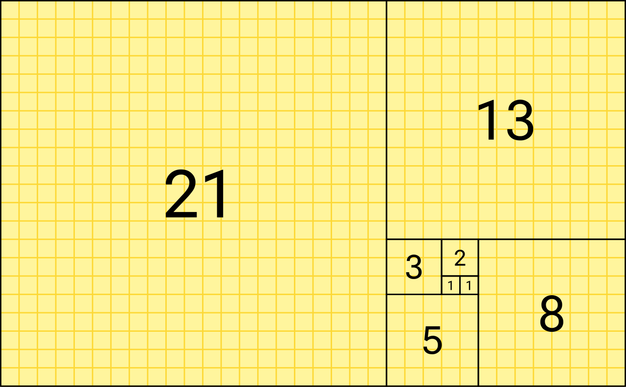
Found in the spiral of galaxies, the arrangement of pinecones, and the family trees of bees, the Fibonacci sequence is a numerical pattern where each term is calculated as the sum of the two immediately preceding terms.
Because you must add two numbers to get the next, the standard Fibonacci sequence begins with the numbers 0,1,1,2,3,5, and 8. (0+1=1, 1+1=2, 1+2=3, 2+3=5, and so on).
Square Numbers
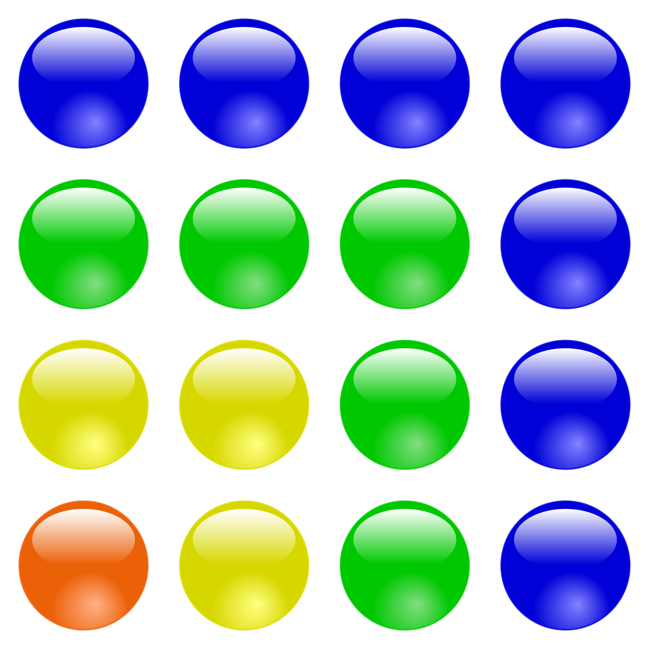
Square numbers form a numerical pattern where every term is the mathematical product of an integer multiplied by itself. Geometrically, these numbers represent the exact quantity of dots needed to form a perfect, filled-in square. The sequence of square numbers begins with the terms 1,4,9,16,25, and 36.
Triangular Numbers
Similar to square numbers, triangular numbers form a numerical pattern representing the total number of dots required to construct progressively larger equilateral triangles. The sequence of triangular numbers begins with the terms 1,3,6,10,15, and 21.
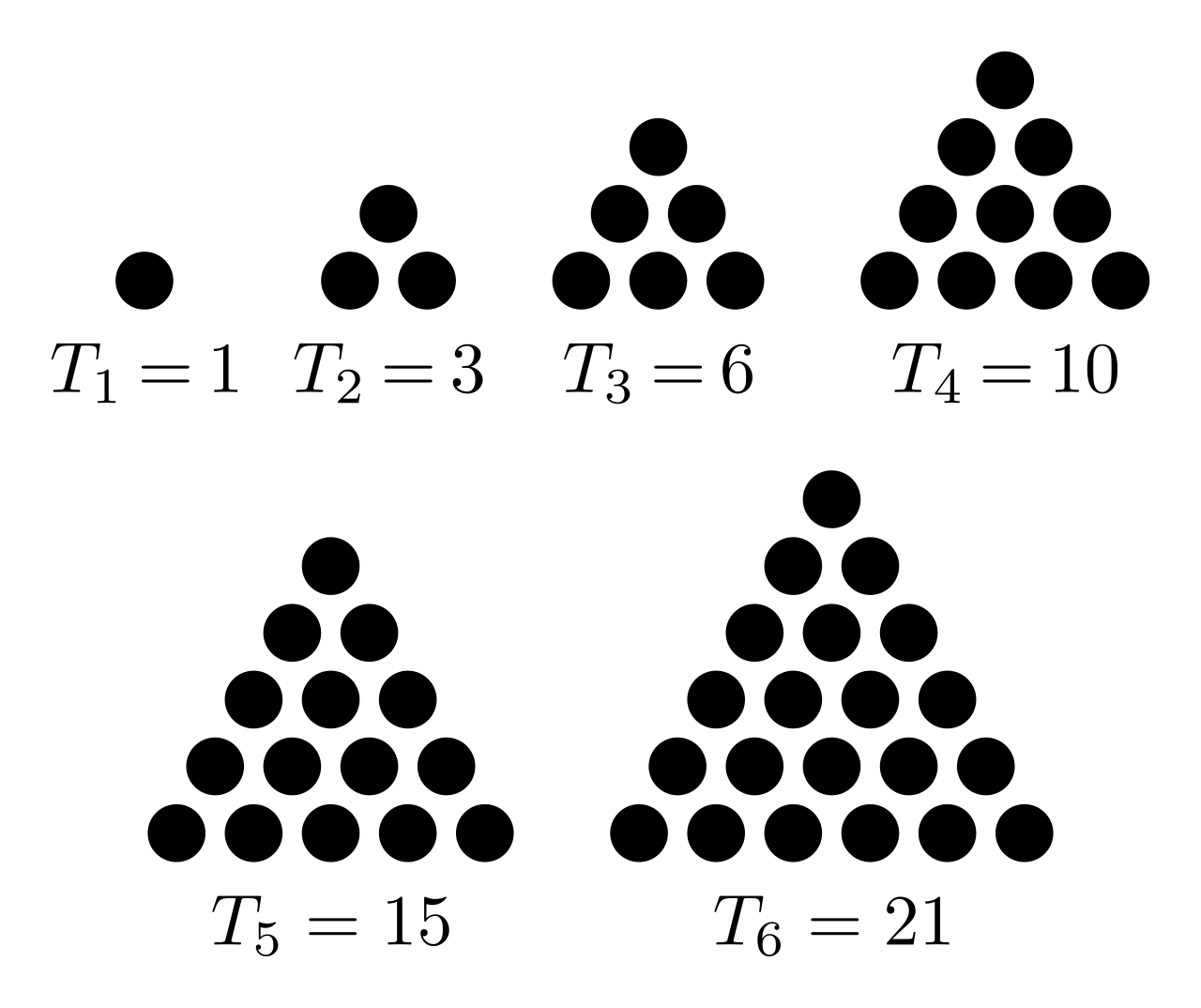
| Position (n) | Triangle Base | Calculation (Sum of integers up to n) | Term |
|---|---|---|---|
| 1st | 1 dot | 1 | 1 |
| 2nd | 2 dots | 1 + 2 | 3 |
| 3rd | 3 dots | 1 + 2 + 3 | 6 |
| 4th | 4 dots | 1 + 2 + 3 + 4 | 10 |
Mathematics thrives on connections. We do not just want to look at one sequence in isolation; we want to see how disparate patterns relate to one another.
The Input-Output Machine
To organize and observe how one value dictates another, we use a tool known as a function table. A function table organizes input and output values to demonstrate the mathematical relationship between two variables.
The mechanism at the heart of this table is the input-output rule, which describes the specific mathematical operation applied to a starting input value to produce the corresponding output value. If the input is 5 and the output is 10, and the input 7 yields output 14, the input-output rule is "multiply by 2."
Comparing Two Patterns
Sometimes, you are tasked with looking at two entirely different sequences generated by separate rules. Identifying a relationship between two separate numerical patterns requires comparing the corresponding terms located in the exact same position in both sequences.
Let us test a specific scenario.
- Pattern A: Starts at 0, Rule is "add 2". (0,2,4,6,8...)
- Pattern B: Starts at 0, Rule is "add 4". (0,4,8,12,16...)
If Pattern A starts at 0 with the rule "add 2" and Pattern B starts at 0 with the rule "add 4", what is the relationship? By comparing the first terms (0 and 0), second terms (2 and 4), and third terms (4 and 8), a beautiful mathematical truth emerges: every term in Pattern B is exactly twice the value of its corresponding term in Pattern A.
Visualizing Relationships: The Coordinate Plane
Once we establish corresponding terms, we have the ingredients for geometry. Corresponding terms from two different numerical patterns can be paired together and written as an ordered pair for graphing.
For the Patterns A and B mentioned above, our ordered pairs (A,B) become: (0,0),(2,4),(4,8),(6,12).
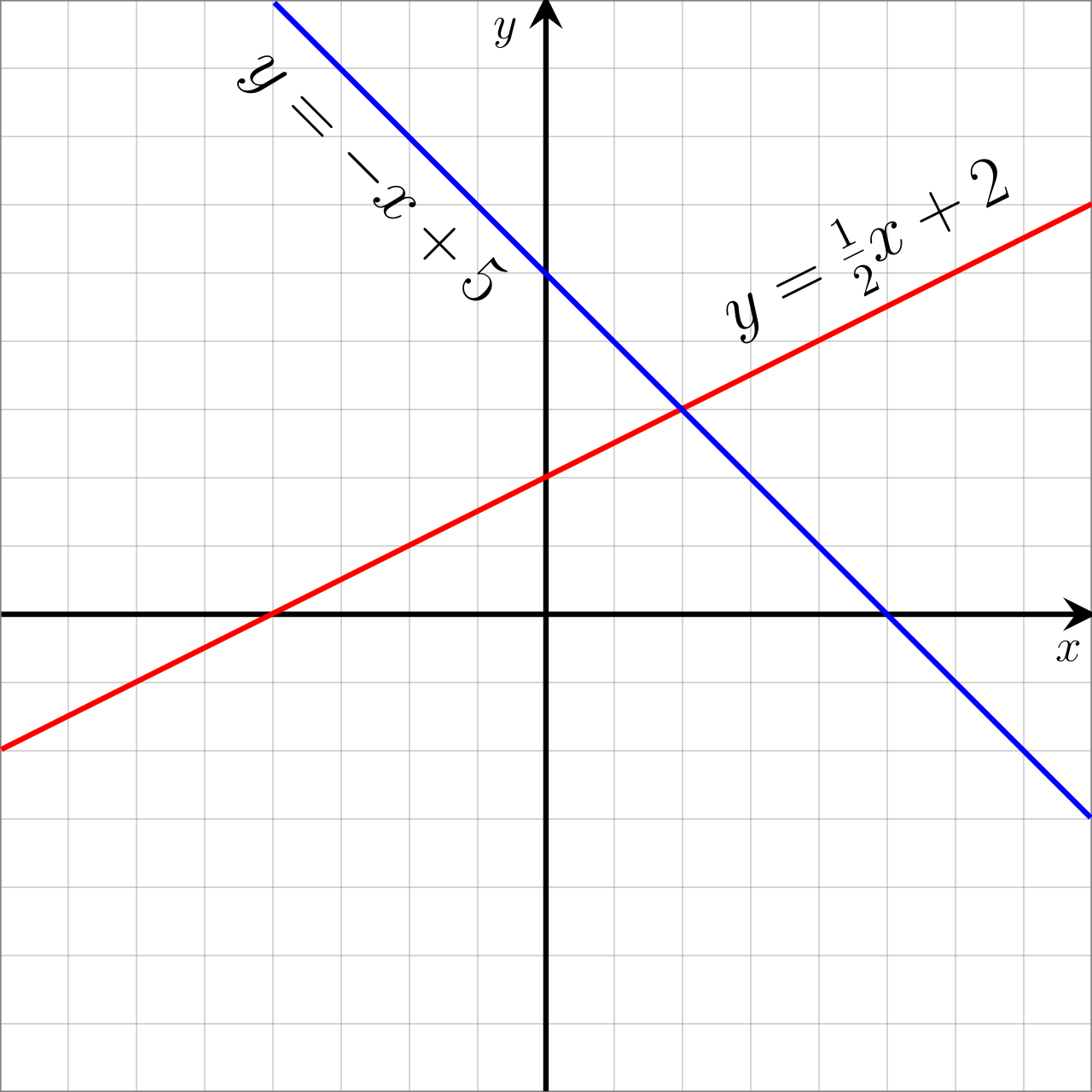
When we transition from numbers to space, magic happens. Graphing ordered pairs generated from two numerical patterns onto a coordinate plane visually demonstrates the proportional or algebraic relationship between the sequences. In the case of Patterns A and B, graphing these pairs yields a perfectly straight line extending from the origin, serving as absolute, irrefutable visual proof of their proportional relationship.
Patterns are not merely a topic to memorize; they are the syntax of mathematics. By learning to recognize, extend, and graph these functions, we are teaching students how to read the blueprint of the logical world.