Analyzing Mathematical Models

Not sure you’re ready?

Take the ~3-minute readiness diagnostic and see where you stand.

When an architect designs a suspension bridge, they do not simply start welding steel over a river. They construct a mathematical model, translating physical tension, wind resistance, and gravity into a system of equations. A mathematical model functions exactly like a blueprint. It strips away the chaotic noise of reality—the rust, the changing weather, the traffic delays—and isolates the essential mechanisms governing a system.

In a real-world mathematical model, the input variable of a function represents the independent quantity—the condition we measure, control, or observe unfolding, such as time elapsed or items produced. The output variable of a function represents the dependent quantity, changing in response to the input. For your future middle school students, the world is a chaotic place. Teaching them to analyze mathematical models is teaching them to find the hidden architecture beneath a cell phone data plan, the trajectory of a tossed basketball, or the compounding spread of a viral video.

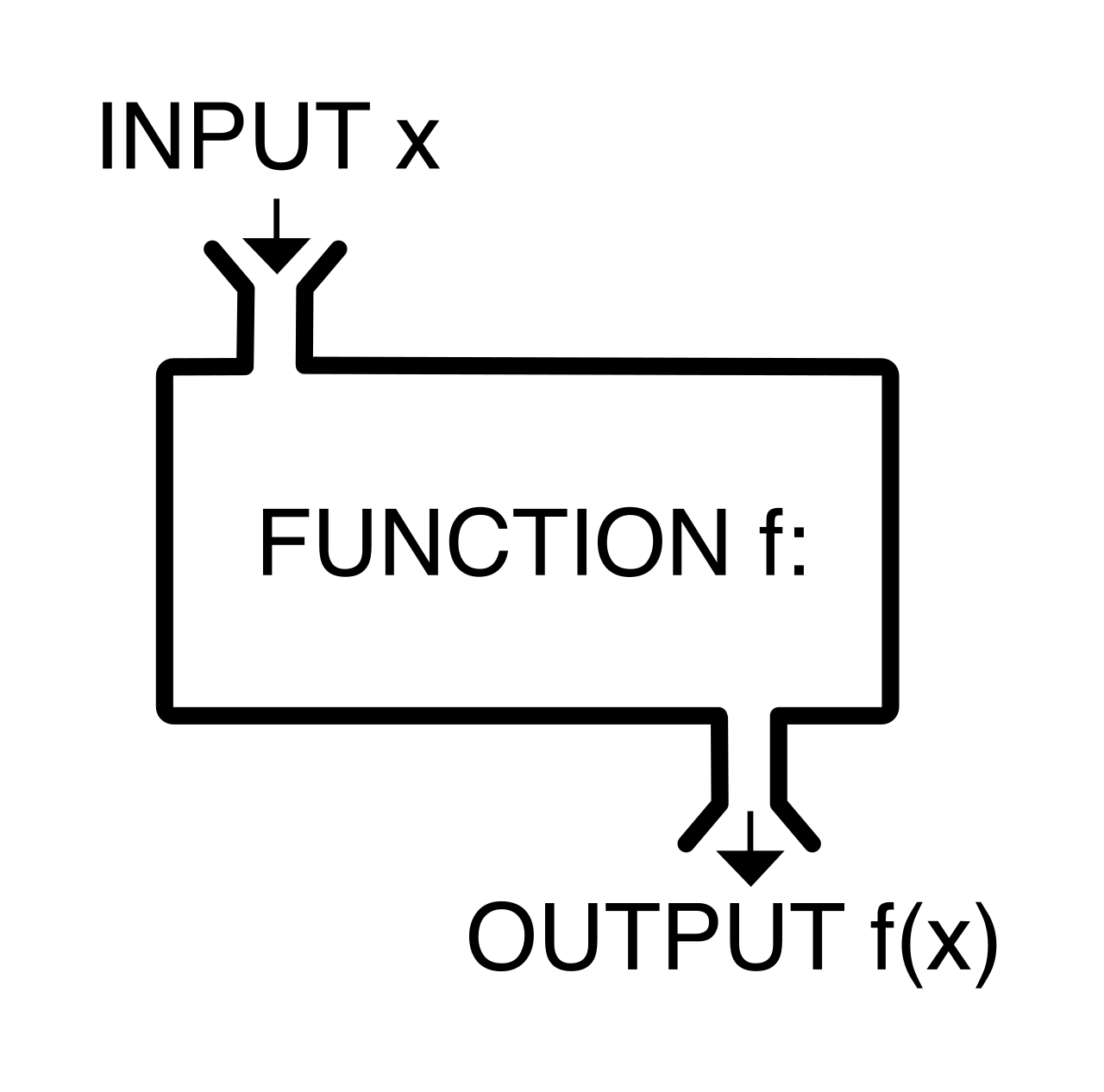
The mathematical function can be visualized as a machine: it takes a specific input variable, applies a consistent mathematical rule, and produces a corresponding output.

To effectively read these mathematical blueprints, we must first master the language they are written in. Many students enter middle school viewing the equals sign merely as a command to "compute the answer." Function notation shifts this paradigm, allowing us to describe complex relationships with high precision.

Function notation $f(x)$ represents the specific output value of a function named $f$ corresponding to an input value of $x$ . It is not multiplication. It is a mapping.

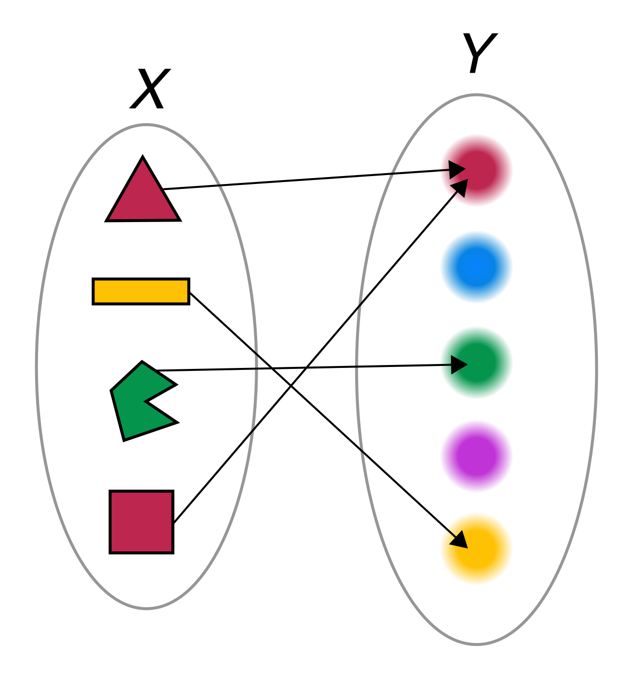
Function notation describes a strict mapping, where each element in the input domain is uniquely assigned to a corresponding output value.

When we write an equation in the form $f(a) = b$ , it signifies that an input of $a$ produces an output of $b$ within the given mathematical context. If $C(t)$ models the cost in dollars of renting a facility for $t$ hours, the statement $C(4) = 150$ is a complete, self-contained sentence: "Renting the facility for 4 hours costs $150." The notation encapsulates both the independent and dependent quantities in a single, readable expression.

If variables $x$ and $y$ are the moving parts of our machine, parameters are the settings on the control board. Parameters in a mathematical model are constants that define the specific characteristics and boundaries of a function for a particular scenario. While variables change continuously within a specific situation, parameters remain locked in place for that situation, dictating how the variables interact.

Let's look at the two foundational models you will teach: linear and exponential functions.

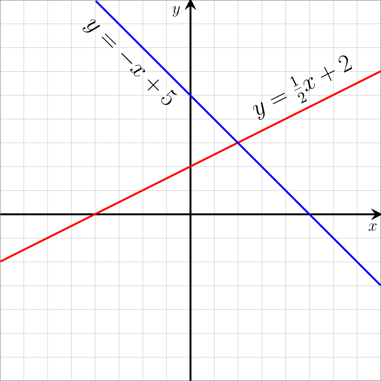
Linear Models: $f(x) = mx + b$

Linear models describe relationships built on constant addition or subtraction.

The parameter $b$ in the linear model $f(x) = mx + b$ represents the initial value of the output when the input quantity is exactly zero. If you are tracking a fundraiser, this might be your starting seed money before any sales are made.
The parameter $m$ in the linear model $f(x) = mx + b$ represents the constant rate of change of the output with respect to the input. It is the steady heartbeat of the model—how much the dependent variable shifts for every single-unit step of the independent variable.

Linear models are defined by a constant average rate of change, meaning the dependent variable shifts by the exact same amount for every unit step of the independent variable.

Exponential Models: $f(x) = a(b)^x$

Exponential models describe relationships built on constant multiplication, commonly seen in population growth, compound interest, or radioactive decay.

The parameter $a$ in the exponential model $f(x) = a(b)^x$ represents the initial amount of the dependent variable when the input is zero.
The parameter $b$ in the exponential model $f(x) = a(b)^x$ represents the constant multiplier or growth factor per unit of the input variable. If $b = 1.05$ , the quantity is growing by 5% per unit of input; if $b = 0.5$ , the quantity is halving.

Exponential growth, such as the replication of a bacterial colony, relies on a constant multiplier rather than constant addition, resulting in a rapidly accelerating curve.

Model Type	Formula	Initial Value Parameter	Growth Parameter	Mechanism of Growth
Linear	$f(x) = mx + b$	$b$	$m$	Constant addition/subtraction
Exponential	$f(x) = a(b)^x$	$a$	$b$	Constant multiplication

How fast is a system evolving? To answer this, we look at the rate of change.

The average rate of change of a function $f(x)$ over a closed interval $[a, b]$ is calculated using the formula: $\frac{f(b) - f(a)}{b - a}$

The average rate of change over an interval is calculated as the change in the dependent variable (vertical axis) divided by the change in the independent variable (horizontal axis), representing the slope of the secant line.

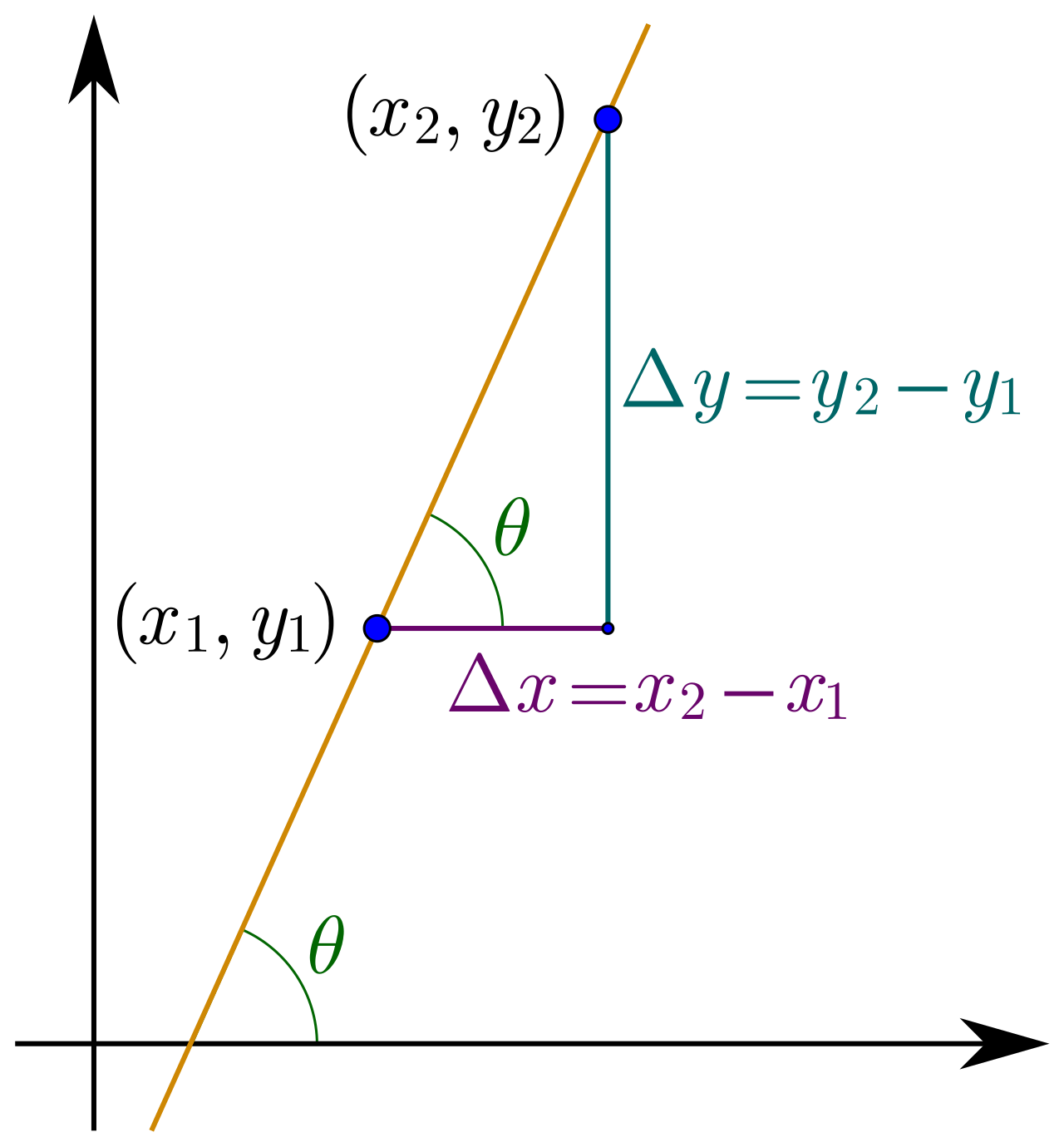
This formula is simply the change in output divided by the change in input. Consequently, the units for an average rate of change are always the units of the output variable divided by the units of the input variable (e.g., dollars per hour, miles per gallon, bacteria per day).

Interpreting the result of this calculation provides immediate insight into the behavior of the model over that specific interval:

A positive average rate of change over an interval indicates that the function's output increases overall from the start of the interval to the end.
A negative average rate of change over an interval indicates that the function's output decreases overall from the start of the interval to the end.
An average rate of change of zero over an interval indicates that the function's starting output and ending output for that interval are identical. (Note: The function may have fluctuated wildly in between, but the net change is zero).

The defining characteristic of linear functions is that they have an identical, constant average rate of change across any chosen interval of their domain. Whether you measure the slope between $x=1$ and $x=2$ , or between $x=10$ and $x=100$ , the result is exactly the same: the parameter $m$ .

In contrast, non-linear functions (like exponential or quadratic models) have average rates of change that vary depending on the specific interval chosen. The growth accelerates or decelerates as the input progresses.

Intercepts are the critical thresholds where mathematical models cross the axes, translating to powerful real-world milestones.

The y-intercept

The y-intercept of a function is the single output value generated when the input variable is equal to exactly zero. Because functions can only have one output for any given input, there can be at most one y-intercept. In contextual time-based models, the y-intercept typically represents the starting point or initial measurement of a scenario before any time elapses. It is the " $t=0$ " moment.

The x-intercepts

The x-intercepts of a function are the specific input values that result in an output of exactly zero. Unlike the y-intercept, a function can have multiple x-intercepts. In contextual physical models, an x-intercept often represents the specific time or condition when a quantity is fully depleted (a bank account hitting $0) or reaches ground level (a falling object hitting the earth).

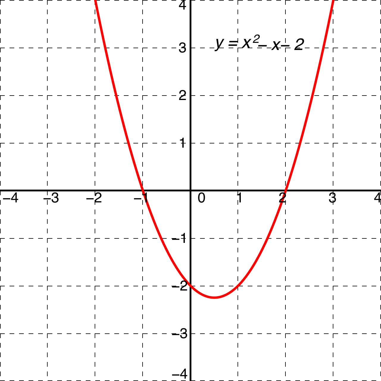
When an object is thrown, launched, or dropped, its trajectory is governed by gravity. This behavior cannot be modeled linearly (because gravity accelerates the object) nor exponentially. It requires a quadratic model.

The standard form of a quadratic function is $f(x) = ax^2 + bx + c$ . Here, the parameter $c$ specifies the exact y-coordinate of the y-intercept. If you evaluate $f(0)$ , the $ax^2$ and $bx$ terms vanish, leaving only $c$ .

To find the x-intercepts of a quadratic model, we must determine when the output is zero. The x-intercepts of a quadratic model can be determined by setting the function equal to zero and solving using factoring, completing the square, or the quadratic formula.

A quadratic mathematical model will display zero, one, or two real x-intercepts depending entirely on the value of the equation's discriminant ( $b^2 - 4ac$ ).

If the discriminant is positive, there are two real x-intercepts.
If the discriminant is zero, there is exactly one real x-intercept (the vertex rests on the x-axis).
If the discriminant is negative, there are zero real x-intercepts (the curve never crosses the axis).

Modeling Projectile Motion

One of the most profound applications of quadratic functions your students will encounter is the projectile motion model. This model predicts the height $h$ of an object at any given time $t$ .

In a quadratic projectile motion model $h(t) = -16t^2 + v_0t + h_0$ , the parameters carry highly specific physical meanings:

The parameter $h_0$ represents the initial height of the object in feet. This is the y-intercept.
The parameter $v_0$ represents the initial vertical velocity of the object in feet per second.

But what about the leading coefficient? The constant $-16$ in the standard English-unit projectile motion function $h(t) = -16t^2 + v_0t + h_0$ is derived from half the acceleration due to Earth's gravity measured in feet per second squared. Earth's gravity pulls objects downward at approximately $32 \text{ ft/s}^2$ . The physics equation for position relies on $\frac{1}{2}gt^2$ , and half of $-32$ is $-16$ .

If you are teaching in a science context, you will likely use the metric system. The constant $-4.9$ in the standard metric-unit projectile motion function $h(t) = -4.9t^2 + v_0t + h_0$ is derived from half the acceleration due to Earth's gravity measured in meters per second squared (gravity is $9.8 \text{ m/s}^2$ , and half of that is $4.9$ ).

When we set this projectile equation to zero and solve for the x-intercepts, we are asking the model: "At what time $t$ is the height $h$ equal to zero?" In almost all real-world contexts, one solution will be negative (representing a theoretical time before the launch, which we discard as outside the practical domain) and one will be positive. The positive x-intercept of a quadratic projectile motion model represents the total amount of time the object remains in the air before hitting the ground.

By mastering these parameters, rates, and intercepts, you equip your students not just to pass an exam, but to mathematically read the physics and phenomena of the world around them.