Comparing Function Types

Not sure you’re ready?

Take the ~3-minute readiness diagnostic and see where you stand.

Place a single water droplet in an empty football stadium, and add one gallon every minute. The water level rises steadily and predictably, etching a perfectly straight line on a graph of volume over time. But if the volume of water doubles every minute—one drop, then two, then four—the early minutes feel deceptively similar to your steady effort. By the time you reach the final few minutes, however, the stadium is inundated in a catastrophic roar of water. This is the profound difference between additive progression and multiplicative explosion, a mathematical distinction that governs the compound interest in a retirement account, the trajectory of a tossed ball, and the spread of a biological population.

As a mathematics teacher, your objective is not simply to teach your students how to plug numbers into formulas. Your objective is to teach them how to read the physical world through the lens of mathematical models. To do this, we must precisely categorize how quantities change.

Nature and human commerce primarily write their laws in three distinct mathematical dialects: linear, quadratic, and exponential. We differentiate these models not merely by looking at the shape of their graphs, but by examining the fundamental mechanism of their growth.

Linear Models: The Engine of Constant Addition

A linear function is the mathematics of a steady march. Fundamentally, a linear function models a situation where a quantity changes at a constant rate per unit interval.

If you are earning a flat hourly wage, or if you are observing a pool drain at a fixed number of gallons per minute, you are witnessing linear change.

The Linear Equation The equation of a linear function can be written in the standard form $f(x) = mx + b$ . Notice that the highest power of the independent variable in a linear function equation is one.

Because the rate of change never wavers, the constant rate of change in a linear function is represented by the slope of the function ( $m$ ). When we plot this relationship on a coordinate plane, the graph of a linear function is a straight line.

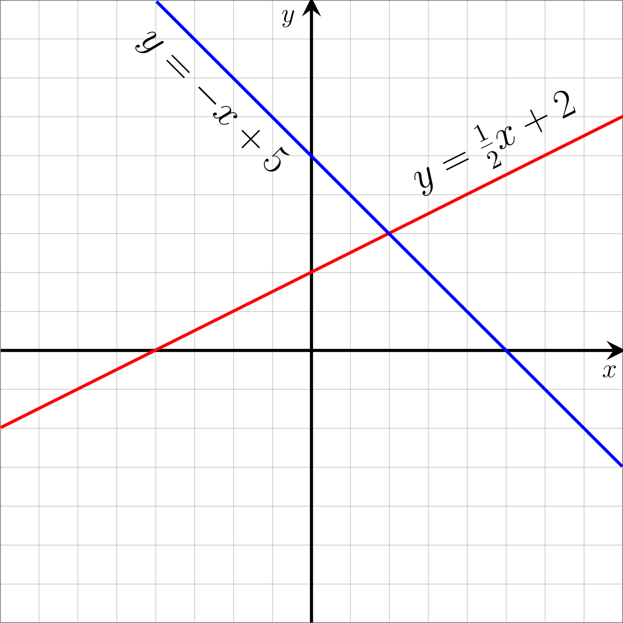
When plotted on a Cartesian plane, linear functions produce perfectly straight lines, representing a constant rate of change without any acceleration or compounding.

How do we spot this in a table of raw data? We look at the gaps between the outputs. For a linear function, the difference between successive y-values is constant for equally spaced x-values. If $x$ increases by $1$ , $y$ might consistently increase by $3$ .

In the realm of finance, simple interest accumulated on a principal amount is modeled by a linear function. If you invest $1,000 at $5\%$ simple interest, you earn exactly $50 every single year. The growth is purely additive.

Quadratic Models: The Engine of Acceleration

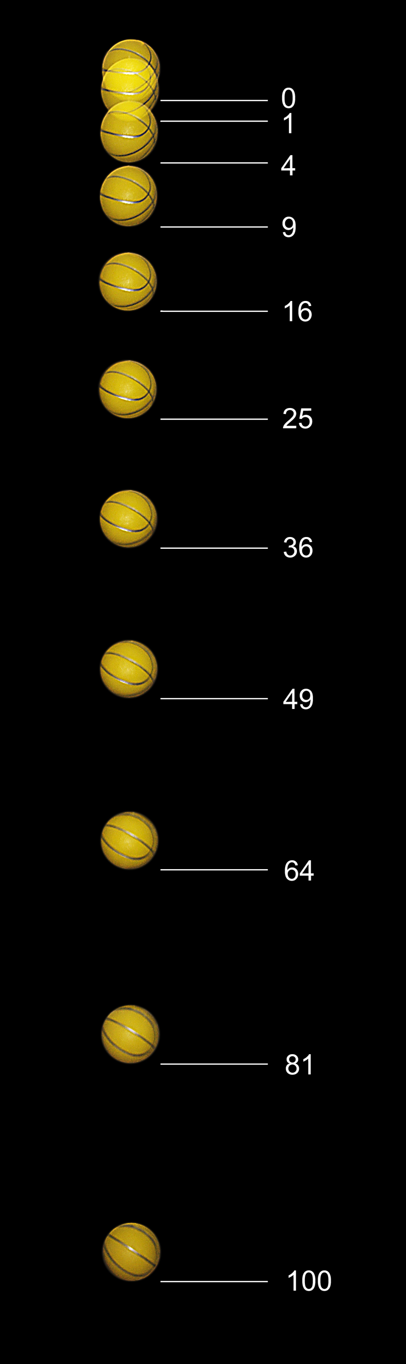
What happens when the rate of change is not constant? If you throw a baseball off a cliff, it does not fall at a steady speed. Uniform gravity pulls on the ball, causing it to speed up as it falls.

A quadratic function models a relationship where the rate of change is not constant. However, this change isn't chaotic; it is highly structured.

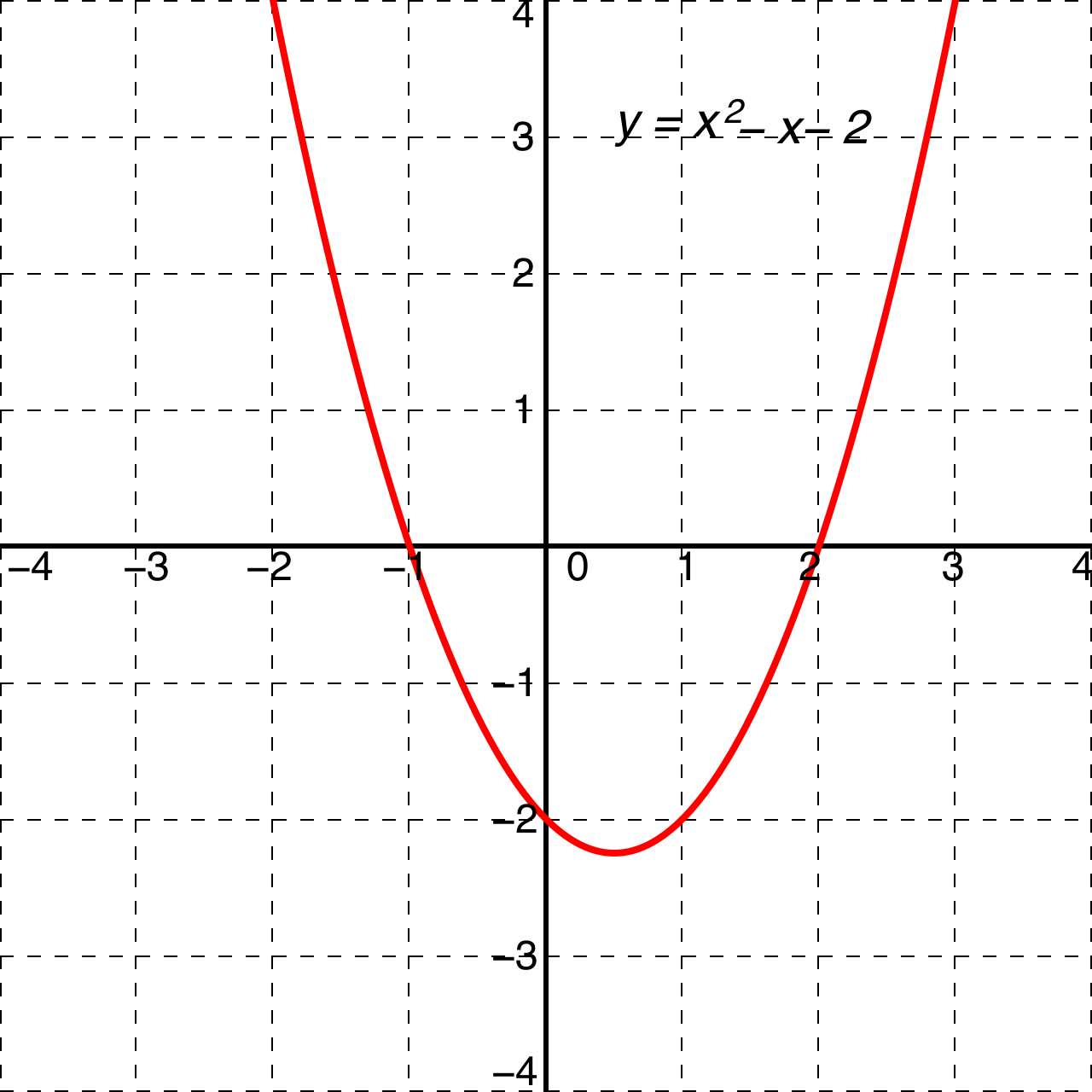
The Quadratic Equation The equation of a quadratic function can be written in the standard form $f(x) = ax^2 + bx + c$ . Here, the highest power of the independent variable in a quadratic function equation is two.

If we look at a table of values for a falling object, the first differences (the changes from one second to the next) will not be constant—they will grow. However, if we take the difference of those differences, a beautiful pattern emerges. For a quadratic function, the second differences of the y-values are constant for equally spaced x-values. This constant second difference perfectly mirrors the constant acceleration of physics. Consequently, the height of a falling object under uniform gravity over time is modeled by a quadratic function.

A freely falling object accelerates uniformly due to gravity. By taking stroboscopic measurements over equal time intervals, we can observe this growing rate of change, which represents a quadratic relationship rather than a linear one.

When plotted on a Cartesian plane, the graph of a quadratic function is a U-shaped curve called a parabola. It bends, reflecting its changing rate of change.

The graph of a quadratic function is a parabola, a symmetrical, U-shaped curve that visually captures the concept of constant acceleration.

Exponential Models: The Engine of Proportions

While linear models grow by constant addition, exponential models grow by constant multiplication. An exponential function models a situation where a quantity changes by a constant percent rate per unit interval.

The Exponential Equation The equation of an exponential function can be written in the standard form $f(x) = a \cdot b^x$ . The defining architectural feature here is that the independent variable in an exponential function equation appears in the exponent.

Because the growth relies on multiplying by a base ( $b$ ), for an exponential function, the quotient of successive y-values is constant for equally spaced x-values. If you divide any $y$ -value by the preceding $y$ -value, you will always get the same number.

The constant ratio between successive y-values in an exponential function is called the growth factor or decay factor.

An exponential function with a base strictly greater than one represents exponential growth. (e.g., $1.05^x$ , which represents a $5\%$ increase).
An exponential function with a base strictly between zero and one represents exponential decay. (e.g., $0.5^x$ , which represents halving).

Exponential models govern profound forces in our universe:

Compound interest accumulated on a principal amount is modeled by an exponential function. Because you earn interest on your interest, your money grows by a constant percent rate (e.g., multiplying your balance by $1.05$ every year).
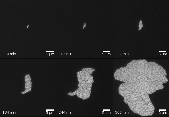
Biological population growth in an environment with unlimited resources is modeled by an exponential function. One bacterium splits into two, two into four, four into eight.

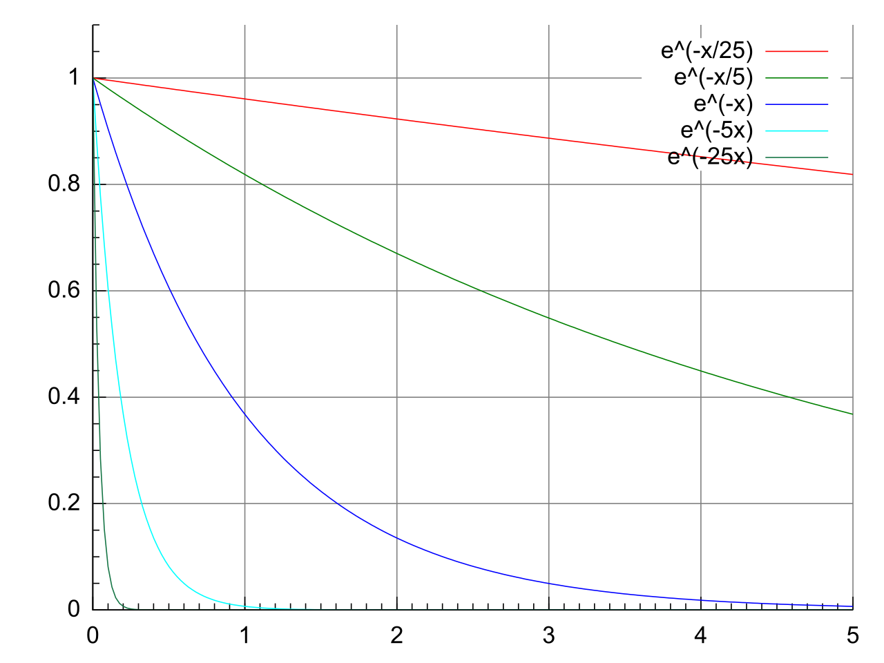
In an environment with ideal conditions, a bacterial population multiplies proportionally over time, visually demonstrating the explosive nature of exponential growth.

The radioactive decay of an isotope over time is modeled by an exponential function. Carbon-14 decays such that half of its mass disappears over a specific time interval, an endlessly halving proportion. As this mass decays infinitesimally closer to zero, we observe its graphical behavior: the graph of an exponential function approaches a horizontal asymptote.

During exponential decay, a quantity endlessly halves by a constant percentage. The resulting graph approaches a horizontal asymptote of zero but mathematically never truly reaches it.

In a middle school classroom, your students will often encounter sequences—lists of numbers—long before they graph continuous functions. It is critical to recognize that these sequences are simply discrete, "stepped" versions of the continuous functions we just defined.

Sequence Type	Defining Trait	Functional Equivalent
Arithmetic Sequence	In an arithmetic sequence, consecutive terms have a constant difference.	Because it grows by constant addition, an arithmetic sequence represents a discrete linear function.
Geometric Sequence	In a geometric sequence, consecutive terms have a constant ratio.	Because it grows by constant multiplication, a geometric sequence represents a discrete exponential function.

If a student understands that an arithmetic sequence (like $5, 8, 11, 14...$ ) is just a set of isolated points lying on a straight line, the leap to $f(x) = 3x + 2$ becomes an intuitive, logical step rather than rote memorization.

One of the most counterintuitive realities your students will face—and one frequently tested on exams—is the long-term behavior of these models. Let's arrange a mathematical race.

Imagine giving a linear function an massive head start. Suppose $f(x) = 1,000,000x$ . Now imagine a seemingly humble exponential function, $g(x) = 1.01^x$ .

At $x = 2$ , the linear function is at $2,000,000$ . The exponential function is at roughly $1.02$ . It looks like no contest. Yet, because the exponential function operates on the principle of self-referential multiplication—its current speed is determined by its current size—it will inevitably, unstoppably accelerate.

It is a strict mathematical law: An exponentially increasing quantity will always eventually exceed a linearly increasing quantity.

What about quadratics? Even a steep parabola like $h(x) = 500x^2$ is fundamentally limited by its degree of two. Its rate of change is growing, but it does so predictably. The exponential function $1.01^x$ , meanwhile, will eventually double, and double, and double again. Therefore, an exponentially increasing quantity will always eventually exceed a quadratically increasing quantity.

If you hand your students a graphing calculator and ask them to adjust the viewing window—zooming out on the x-axis to $100$ , then $1,000$ , then $10,000$ —they will witness the parabola visually collapse beneath the sheer vertical wall of the exponential curve.

Understanding this hierarchy—that constant addition (linear) is trumped by increasing addition (quadratic), which is ultimately obliterated by proportional multiplication (exponential)—is the keystone to mastering algebraic modeling. When you teach this, you aren't just teaching exam requirements; you are providing the key to understanding the architecture of change itself.