Relationships Among Functions, Tables, and Graphs

Not sure you’re ready?

Take the ~3-minute readiness diagnostic and see where you stand.

A mathematical function leaves three distinct footprints in the physical world: a rule (the equation), a ledger (the table), and a photograph (the graph). To understand a function deeply is to learn the art of translating freely among these representations. As an aspiring middle school mathematics teacher, your task goes beyond merely calculating values; you are teaching students to read the "DNA" of an equation and predict its visual reality on a coordinate plane. When a student can look at a table of numbers and visualize the curve it traces before even powering on their graphing calculator, they have grasped the profound relationship between algebra and geometry.

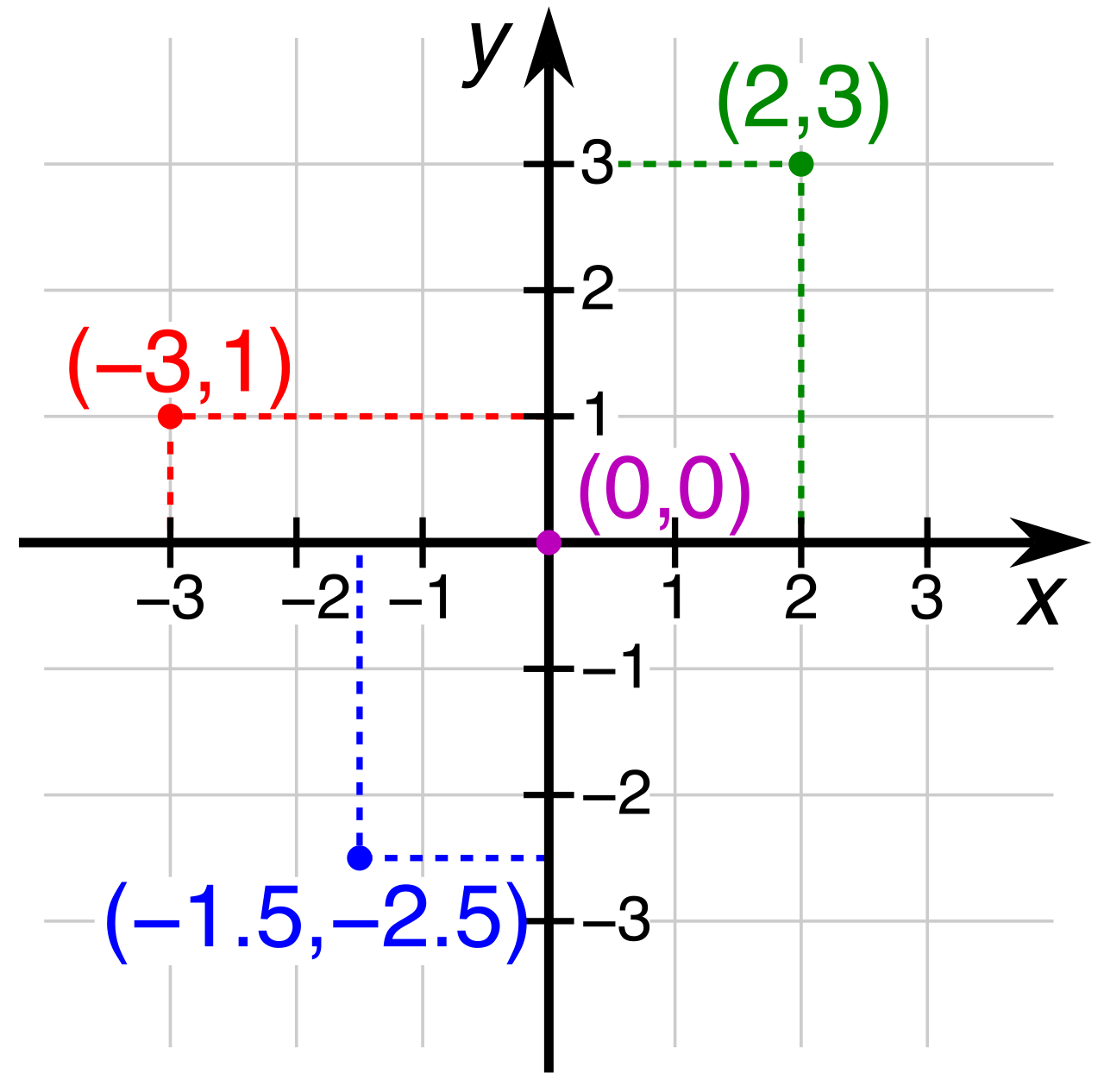
A Cartesian coordinate plane illustrating the geometric space where mathematical functions are graphed and analyzed.

Before we can build complex mathematical structures, we must understand the straight line. The defining characteristic of a linear function is its unwavering consistency.

Reading the Ledger: Tables and Intercepts

We can diagnose the nature of a function simply by observing its outputs. A table of values represents a linear function if the first differences between consecutive $y$ -values are constant for equally spaced $x$ -values. This unyielding constant rate of change is the heartbeat of a linear relationship.

When analyzing any functional table, the origin points—the intercepts—serve as our geographical anchors. The $y$ -intercept of a function's graph corresponds to the ordered pair in a table where the $x$ -value is exactly zero. Conversely, the $x$ -intercepts of a function's graph correspond to the ordered pairs in a table where the $y$ -value is exactly zero. Teaching students to immediately scan a table for zeros empowers them to instantly locate the graph's intersection with the axes.

Measuring the Incline: Slope

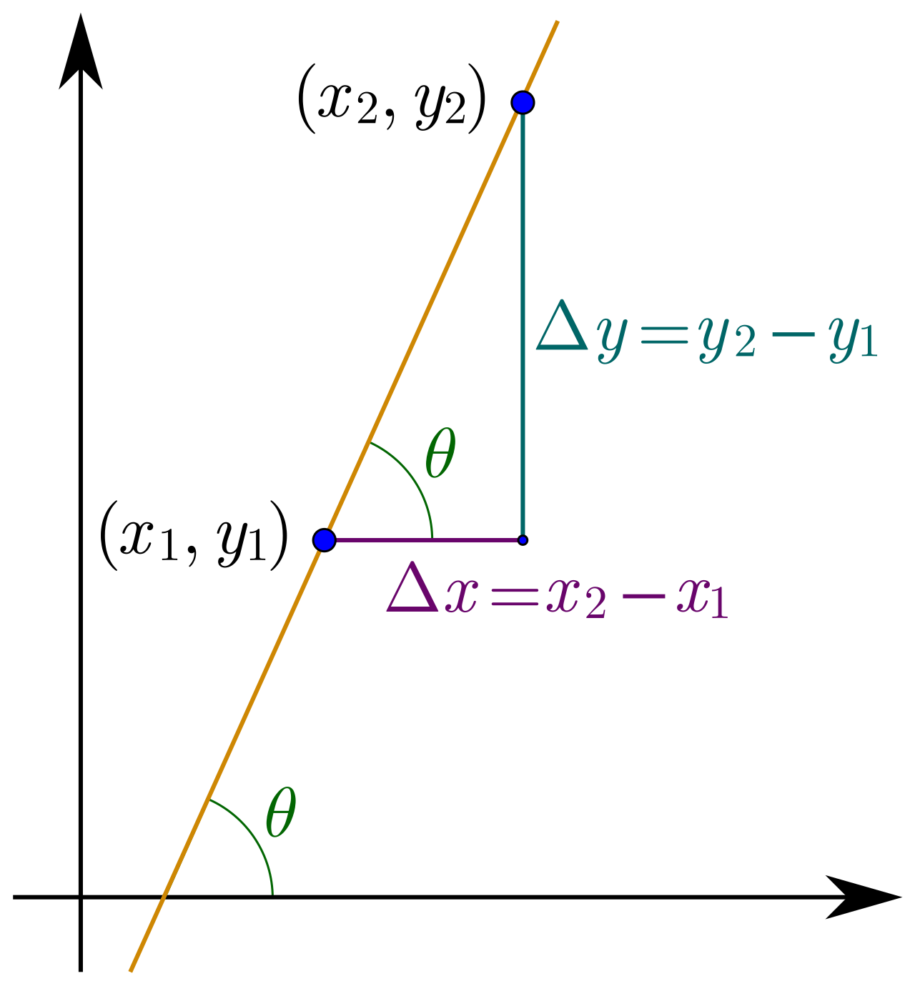
This constant rate of change we observe in the table is mathematically formalized as the slope. The slope of a linear function can be calculated from a table or graph by dividing the change in vertical $y$ -values by the corresponding change in horizontal $x$ -values between any two points. It is a ratio of physical movement—how far the graph rises or falls relative to how far it runs.

Slope is calculated as the ratio of the vertical change (rise) to the horizontal change (run) between any two points on a line.

The Equations: Blueprints of a Line

Lines are governed by highly efficient equations, primarily encountered in two forms:

Slope-Intercept Form: $y = mx + b$ In the slope-intercept form $y = mx + b$ , the variable $m$ represents the slope of the line, dictating its steepness and direction. Furthermore, in the slope-intercept form $y = mx + b$ , the variable $b$ represents the $y$ -coordinate of the $y$ -intercept. This form is uniquely powerful for immediate graphing.

Point-Slope Form: $y - y_1 = m(x - x_1)$ In the point-slope form $y - y_1 = m(x - x_1)$ , the variables $x_1$ and $y_1$ represent the coordinates of a specific known point on the line. This is the working mathematician's equation; it allows us to construct a line algebraically the moment we know its slope and any single point it passes through, without needing to calculate the $y$ -intercept first.

When the rate of change is no longer constant, the straight line bends. The graph of a quadratic function is a U-shaped curve called a parabola.

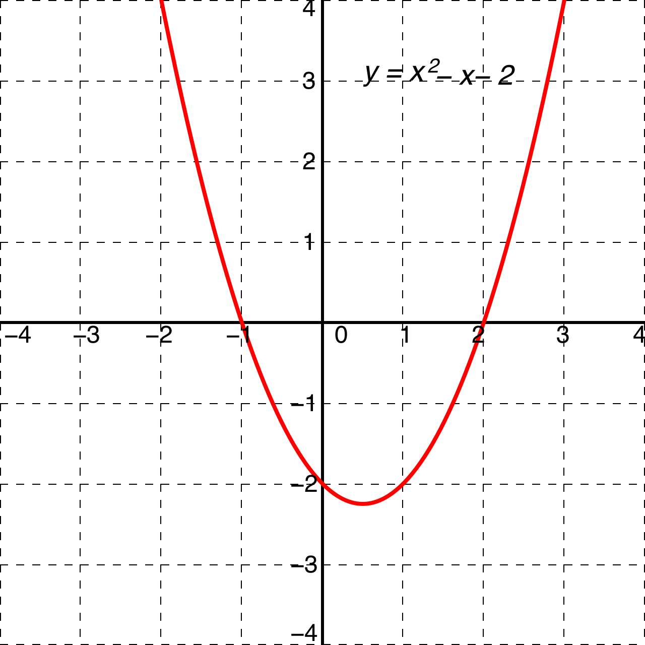
The graph of a quadratic function forms a parabola, a U-shaped curve that can cross the x-axis to reveal the function's roots.

How do we detect this curve mathematically? We return to our ledger. A table of values represents a quadratic function if the second differences between consecutive $y$ -values are constant for equally spaced $x$ -values. The rate of change is itself changing at a constant rate, mimicking the physics of gravity and acceleration.

Quadratic functions offer a rich landscape of symbolic representations. The form in which a quadratic equation is written dictates precisely which graphical feature is immediately visible.

Form	Equation	Key Insights Revealed
Standard	$y = ax^2 + bx + c$	In the standard quadratic form $y = ax^2 + bx + c$ , the variable $c$ represents the $y$ -coordinate of the $y$ -intercept. Additionally, the axis of symmetry of a parabola given in standard form $y = ax^2 + bx + c$ is the vertical line defined by the equation $x = -b / (2a)$ .
Factored / Intercept	$y = a(x - p)(x - q)$	The factored form or intercept form of a quadratic equation is $y = a(x - p)(x - q)$ . In the factored quadratic form $y = a(x - p)(x - q)$ , the variables $p$ and $q$ represent the $x$ -coordinates of the $x$ -intercepts.
Vertex	$y = a(x - h)^2 + k$	The vertex form of a quadratic equation is $y = a(x - h)^2 + k$ . In the quadratic vertex form $y = a(x - h)^2 + k$ , the variables $h$ and $k$ represent the coordinates of the parabola's vertex at point $(h, k)$ .

Notice a recurring character in all three forms: the leading coefficient, $a$ . The variable $a$ in the quadratic vertex form $y = a(x - h)^2 + k$ determines the direction of the parabola's opening and its vertical stretch or compression.

Its sign dictates the geometry of the curve:

A positive value of the leading coefficient $a$ in a quadratic equation causes the parabola to open upward, creating a definitive minimum point.
A negative value of the leading coefficient $a$ in a quadratic equation causes the parabola to open downward, arching over to create a maximum peak.

Beyond linear and quadratic functions, middle school mathematics introduces families of functions that expand a student's analytical toolkit. Every complex function is merely a modification of a simple "parent" function.

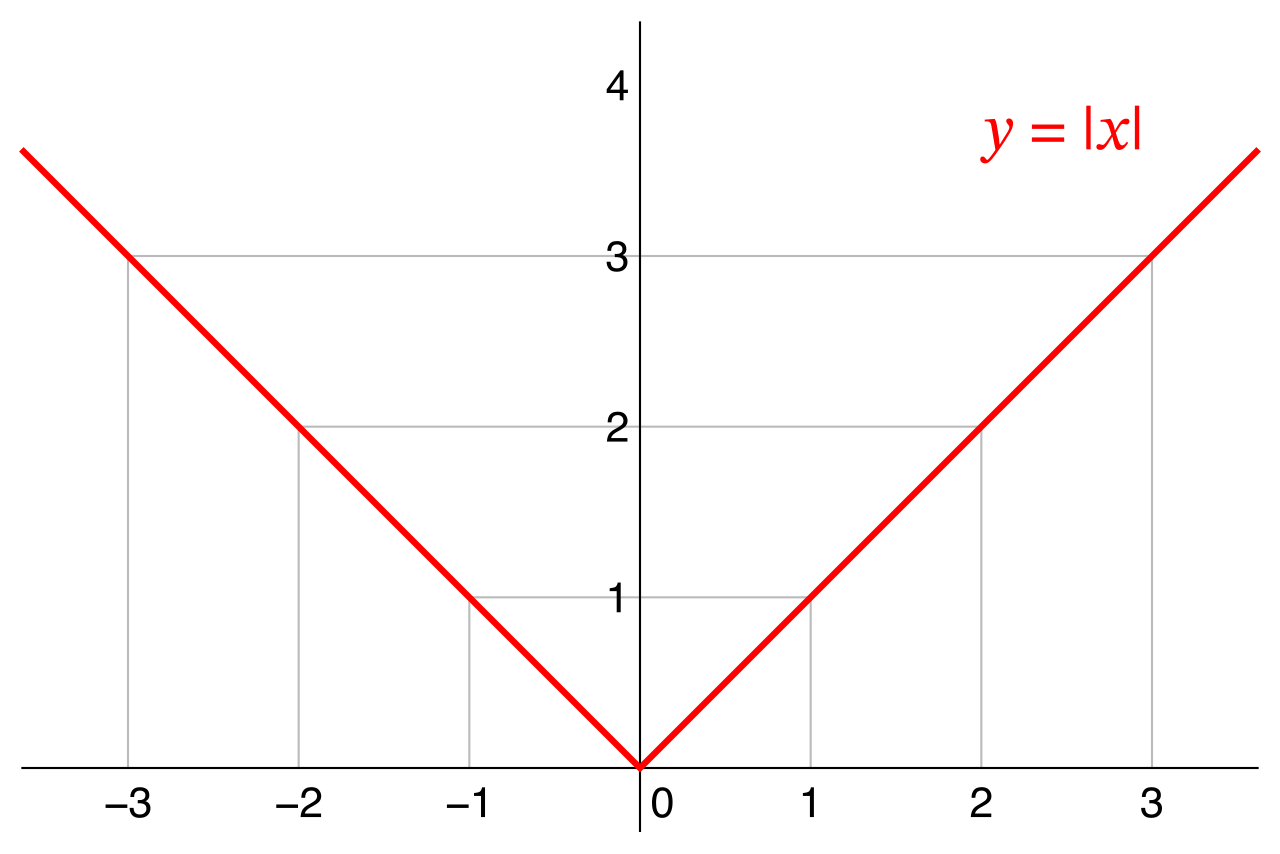
The Absolute Value Function The parent absolute value function is $f(x) = |x|$ . Because absolute value measures distance from zero—a strictly non-negative quantity—the graph of the parent absolute value function $f(x) = |x|$ has a V-shape with its vertex situated at the origin $(0,0)$ . For positive inputs, it behaves like $y = x$ ; for negative inputs, it reflects upwards, mimicking $y = -x$ .

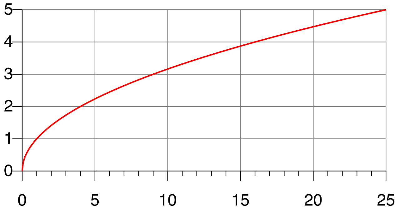
The parent absolute value function, f(x) = |x|, forms a characteristic V-shape with its vertex at the origin.

The Square Root Function The parent square root function is $f(x) = \sqrt{x}$ . Unlike linear or absolute value functions, which accept any real number as an input, the square root has boundaries. The domain of the parent square root function $f(x) = \sqrt{x}$ is restricted to all non-negative real numbers, because the square root of a negative number is not a real number. Consequently, the graph of the parent square root function $f(x) = \sqrt{x}$ begins at the origin $(0,0)$ and curves outward into the first quadrant, slowly flattening as $x$ increases.

The parent square root function, f(x) = √x, begins at the origin and curves outward exclusively within the non-negative first quadrant.

One of the most elegant discoveries in mathematics is that the rules for moving a line are the exact same rules for moving a parabola, a V-shape, or a square root curve. We call these universal rules transformations.

Translations: Shifting the Grid

A translation is a rigid motion. A vertical translation shifts the entire graph of a function upward or downward without altering the graph's overall shape or orientation. This occurs when we modify the output of the function.

Adding a positive constant $k$ to the output of a function, written as $f(x) + k$ , translates the graph vertically upward by $k$ units.
Subtracting a positive constant $k$ from the output of a function, written as $f(x) - k$ , translates the graph vertically downward by $k$ units.

A horizontal translation shifts the entire graph of a function to the left or right without altering the graph's overall shape or orientation. This occurs when we modify the input directly. For students, horizontal translations often feel counter-intuitive.

Subtracting a positive constant $h$ from the input variable of a function, written as $f(x - h)$ , translates the graph horizontally to the right by $h$ units.
Adding a positive constant $h$ to the input variable of a function, written as $f(x + h)$ , translates the graph horizontally to the left by $h$ units.

Why is it reversed? If an original function achieved its vertex when the input was $0$ , the new function $f(x - 3)$ requires $x$ to be $3$ to achieve that exact same zero state (since $3 - 3 = 0$ ). Thus, the entire graph must step $3$ units to the right.

A translation slides a graph horizontally or vertically across the coordinate plane without altering its original shape or orientation.

Reflections: The Mathematical Mirror

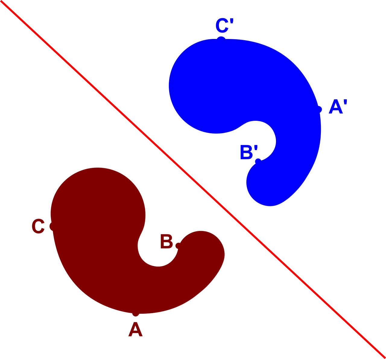
Reflections create mirror images of a graph across an axis. The placement of a negative sign completely changes the axis of reflection.

A reflection of a function over the x-axis transforms the symbolic representation of the function $f(x)$ into $-f(x)$ . Multiplying a function's entire output by negative one visually flips the graph vertically across the horizontal x-axis. All positive heights become negative depths.
A reflection of a function over the y-axis transforms the symbolic representation of the function $f(x)$ into $f(-x)$ . Multiplying a function's input variable by negative one visually flips the graph horizontally across the vertical y-axis. The future becomes the past.

A reflection acts as a mathematical mirror, flipping a function's graph across an axis to create its symmetrical image.

Dilations: Stretches and Compressions

Finally, we can warp the space a function occupies by multiplying it by a scalar factor.

A vertical stretch occurs when a function is multiplied by a constant factor $a$ , provided the absolute value of $a$ is greater than 1 ( $|a| > 1$ ). The outputs are magnified; the $y$ -values climb faster, and the graph appears narrower or taller.
A vertical compression occurs when a function is multiplied by a constant factor $a$ , provided the absolute value of $a$ is strictly between $0$ and $1$ ( $0 < |a| < 1$ ). The outputs are diminished; the graph flattens, expanding outward as the $y$ -values take longer to grow.

By mastering these architectural rules, you ensure your students are never memorizing isolated graphs. They are learning a universal geometric language—a master key that unlocks every functional relationship they will encounter from middle school through calculus.