Linear Models and Bivariate Data
Not sure you’re ready?
Take the ~3-minute readiness diagnostic and see where you stand.
Imagine tracking the exact number of hours a group of middle school students spends practicing algebra problems, and pairing each time with their respective scores on a final exam. You are no longer looking at a single, isolated list of grades; you are examining bivariate measurement data, which consists of observations of two different quantitative variables for each subject. To make sense of this paired information, you plot it. A scatterplot is a graphical representation used to display bivariate quantitative data on a coordinate plane. The rule of mapping is strict and logical: the independent driver, or the explanatory variable, is plotted along the horizontal x-axis, while the measured outcome, or the response variable, is plotted along the vertical y-axis. By mapping data this way, we transform a chaotic spreadsheet into a visual narrative.
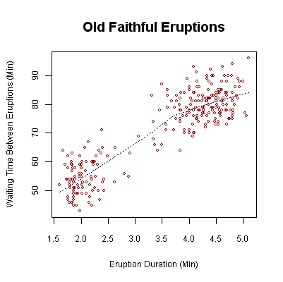
When we look at a scatterplot, we are searching for a story in the noise. We evaluate this story by observing three distinct characteristics of the association between the variables: form, direction, and strength.
The form of an association describes whether the overall pattern of the data points is linear or nonlinear. For our purposes, we are primarily interested in linear forms—data that generally clusters along a straight path.
If the form is linear, we then determine its direction. The direction of an association in a scatterplot can be classified as positive or negative.
- A positive association means the response variable tends to increase as the explanatory variable increases. Think of the relationship between hours spent studying and exam scores.
- A negative association means the response variable tends to decrease as the explanatory variable increases. Consider the relationship between the weeks a new smartphone has been on the market and its resale value.
Finally, we assess the strength of an association, which describes how closely the data points follow a clear pattern or trend. If the points are tightly packed along an invisible line, the association is strong. If they resemble a loose cloud, it is weak.
Anomalies: Outliers and Influential Points
Reality is rarely perfectly tidy. Data often contains anomalies that deviate from the primary narrative.
An outlier in bivariate data is a point that falls far outside the overall pattern of the other data points. If a student studied for 15 hours but scored a 30% on the exam, that point defies the general positive trend. It is an outlier.
However, there is a specialized class of anomaly known as an influential point. An influential point is a data point whose removal significantly changes the slope or y-intercept of the line of best fit.
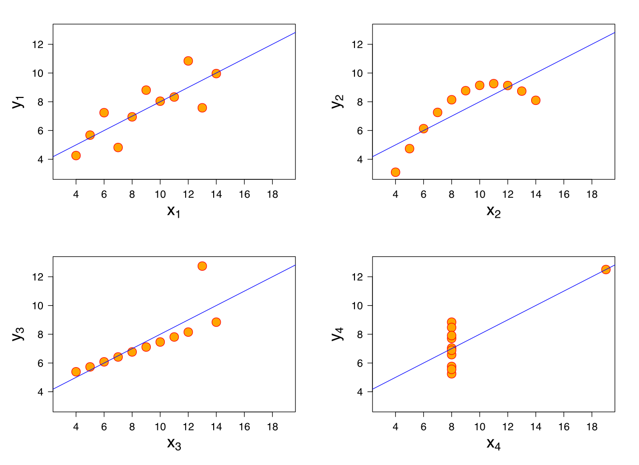
The Seesaw Analogy: Imagine a scatterplot as a seesaw. A point placed far out on the extreme left or right of the x-axis has incredible leverage. If that point breaks the pattern, it will drag the entire regression line toward itself. Conversely, an outlier sitting dead-center on the x-axis but very high on the y-axis might raise the whole line slightly, but it won't drastically tilt the slope. Only the point with high leverage that pulls the line significantly is deemed an influential point.
While describing a scatterplot visually is helpful, mathematics demands precision. We need a numerical index to measure how tightly our variables are tethered together.
Correlation is a statistical measure quantifying the strength and direction of a linear relationship between two quantitative variables. To express this, we use a specific metric: the Pearson correlation coefficient, mathematically denoted by the lowercase letter r.
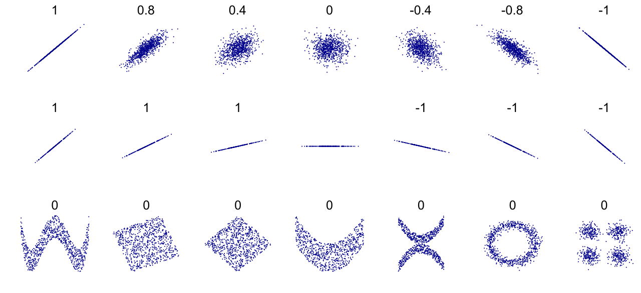
The value of the correlation coefficient r always falls between negative one and positive one inclusive (−1≤r≤1).
| Value of r | Interpretation |
|---|---|
| Exactly 1 | Indicates a perfect positive linear relationship. Every point falls exactly on an upward-sloping line. |
| Exactly -1 | Indicates a perfect negative linear relationship. Every point falls exactly on a downward-sloping line. |
| 0 | Indicates the complete absence of a linear relationship between two variables. The points look like shotgun spray. |
The closer ∣r∣ is to 1, the stronger the linear association. A correlation of 0.85 is strong; a correlation of 0.12 is incredibly weak.
The Golden Rule of Statistics
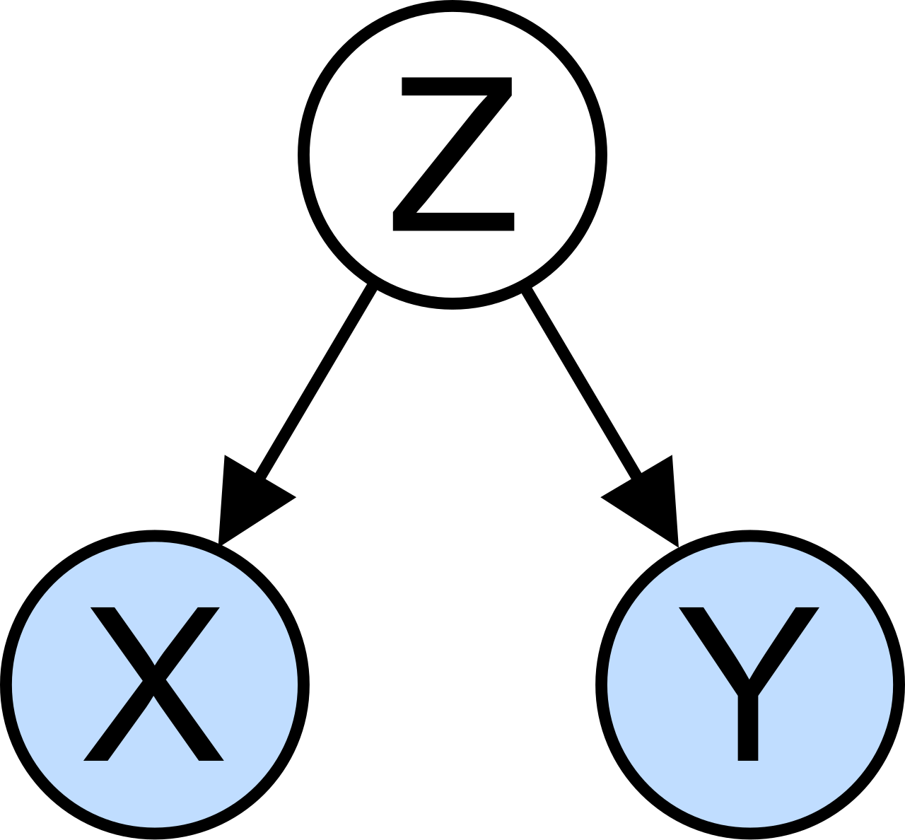
As educators, this is arguably the most vital concept you must impart to your future students: Correlation between two variables does not prove that a causal relationship exists between those variables.
If you graph the monthly sales of ice cream against the number of shark attacks at the beach, you will find a strong positive correlation (r is high). Does eating ice cream attract sharks? Of course not. Both variables are responding to a hidden, "confounding" variable: summer weather. Correlation is merely an observation that two variables move together; causation is the rigorous proof that one actively forces the other to move.
Once we establish that two variables have a strong linear correlation, we want to build a mathematical bridge between them. We do this by calculating a line of best fit, which is a straight line drawn through the center of the data points on a scatterplot to model a linear trend.
But how do we know our line is truly the "best"? Why not tilt it slightly up or down? We judge the quality of a line by examining its errors, known mathematically as residuals.
A residual is the vertical distance between an observed data point and the predicted value on a line of best fit. It is literally the error of our prediction.
Calculating a Residual: Residual=Observed y−Predicted y
Because we are subtracting the prediction from reality, the mathematical sign of the residual tells us exactly where the true data point lies in space:
- A positive residual indicates that the observed data point lies above the line of best fit. Reality exceeded expectations.
- A negative residual indicates that the observed data point lies below the line of best fit. The prediction was an overestimate.
- A residual of zero indicates that the observed data point lies exactly on the line of best fit. The prediction was flawless.
The Least-Squares Regression Line
If we draw a line through a scatterplot, we will create many residuals—some positive, some negative. The ultimate goal is to minimize these errors. The least-squares regression line is the specific line of best fit that minimizes the sum of the squared residuals.
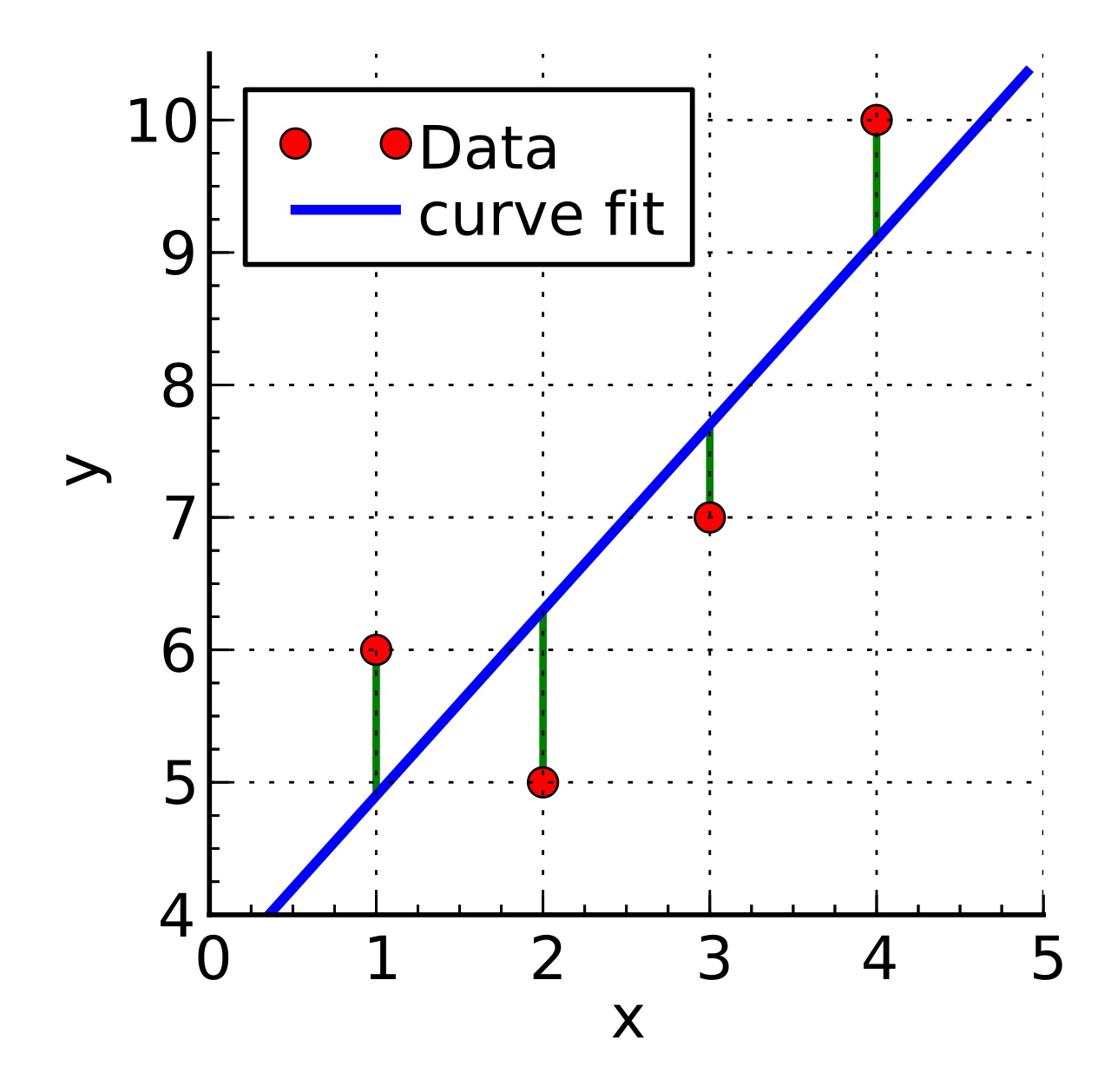
Why do we square them? If we simply added up raw residuals, large positive errors and large negative errors would cancel each other out, falsely suggesting the line is a great fit. Squaring makes all errors positive, fiercely penalizing large deviations. The least-squares regression line minimizes this total squared error, finding the exact mathematical center of the data.
Because it is the perfect center of mass, a fascinating mathematical property emerges: The sum of all residuals for a least-squares regression line is always exactly zero. The positive errors perfectly balance the negative errors.
When we calculate this least-squares regression line, we express it using the familiar linear equation: y=mx+b.
In this equation, the variable m represents the slope of the line, and the variable b represents the y-intercept. However, on your exam—and in your classroom—you must move beyond algebra into statistical interpretation.
Interpreting the Slope
The slope of a linear model represents the predicted change in the response variable for every one-unit increase in the explanatory variable.
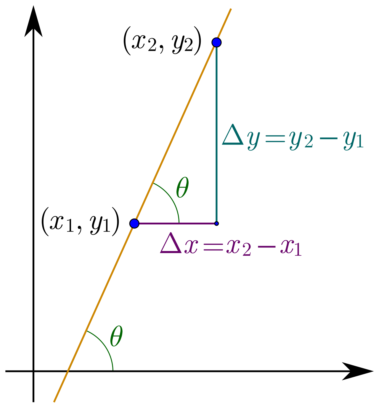
Imagine a model predicting a student's final exam score (y) based on hours studied (x): y=4.5x+50. The slope is 4.5. You must interpret this precisely: "For every additional one hour of studying, the predicted final exam score increases by 4.5 points." (Notice the crucial inclusion of the word "predicted." We are modeling a trend, not stating a guarantee).
Furthermore, the slope and correlation are deeply intertwined. The slope of the least-squares regression line always has the same mathematical sign as the correlation coefficient r. If r is positive, the slope m is positive. If r is negative, m is negative.
Interpreting the Y-Intercept
The y-intercept of a linear model represents the predicted value of the response variable when the explanatory variable is exactly zero.
In our studying model (y=4.5x+50), the y-intercept is 50. The interpretation is straightforward: "If a student studies for zero hours, their predicted final exam score is 50."
However, context is everything. The y-intercept of a linear model may lack a meaningful real-world interpretation if an explanatory value of zero is impossible or completely outside the bounds of reason. Suppose you have a model predicting a middle schooler's height (y, in inches) based on their weight (x, in pounds): y=0.2x+40. The intercept tells us that a student weighing exactly 0 pounds is predicted to be 40 inches tall. A student weighing zero pounds does not exist. In this case, the y-intercept is strictly a mathematical anchor for the line, completely devoid of real-world meaning.
The greatest power of an equation is its predictive capability. A line of best fit can be used to predict the value of a response variable for a given value of an explanatory variable.
Predictions using a linear model are calculated by substituting a specific input value into the linear equation to solve for the output value. If we want to predict the exam score of a student who studied for 4 hours using y=4.5x+50, we substitute 4 for x: y=4.5(4)+50=18+50=68. The predicted score is 68.
When we make predictions, we engage in one of two practices: interpolation or extrapolation.
Interpolation is the process of using a model to predict a value within the range of the observed explanatory variables. If our original data included students who studied anywhere from 1 to 10 hours, predicting the score for a student who studied for 4 hours is interpolation. It is mathematically safe and logically sound.
Extrapolation is the process of using a model to predict a value outside the range of the observed explanatory variables. If we use the exact same equation to predict the score of a student who studied for 20 hours, we substitute 20 for x: y=4.5(20)+50=90+50=140. The exam is only out of 100 points. The prediction broke.
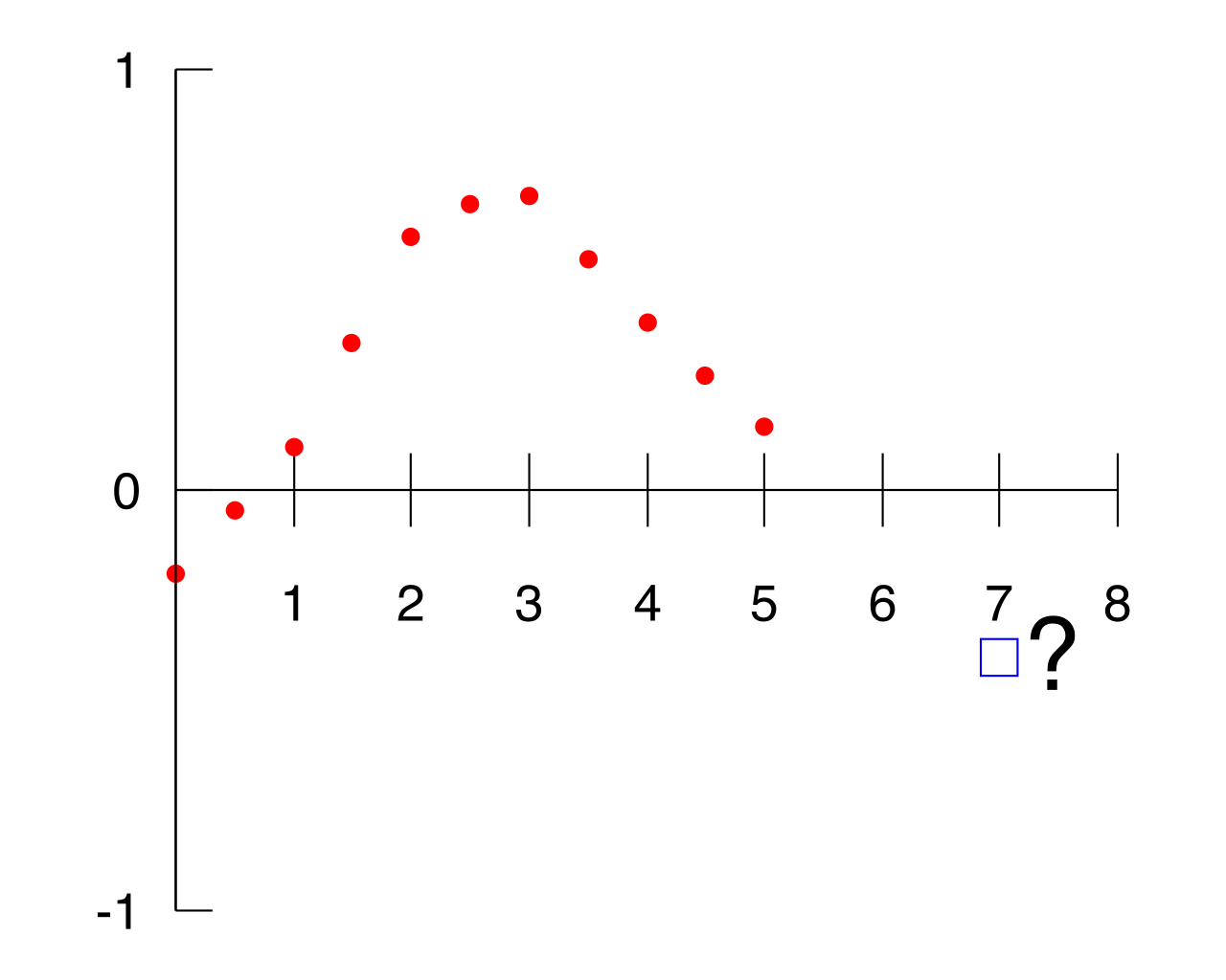
This highlights a critical limitation: Extrapolating beyond the range of observed data often produces unreliable predictions. Relationships between variables rarely stay perfectly linear forever. The growth of a plant might be linear for its first three weeks, but if you use that linear model to extrapolate its height at ten years old, the math will confidently predict a plant that reaches the stratosphere.
When you stand before your students, bivariate data shouldn't be taught merely as points on a grid. It is the geometry of relationships. It is how we quantify how one aspect of our world influences another.
By understanding the visual form (scatterplots), measuring the strength (correlation), computing the trend (least-squares regression), analyzing the errors (residuals), and respecting the boundaries (interpolation vs. extrapolation), you equip your students with the most powerful tool in modern applied mathematics: the ability to observe the past and accurately predict the future.