Data Displays and Relative Frequencies

Not sure you’re ready?

Take the ~3-minute readiness diagnostic and see where you stand.

A school administrator hands you a spreadsheet containing the test scores, lunch preferences, and attendance records of four hundred seventh graders. Staring at the raw rows and columns reveals almost nothing. Human cognition is not built to parse infinite grids of symbols; we are visual creatures. To understand the story hidden within a dataset, we must translate numbers and labels into physical dimensions—lengths, areas, and angles.

A spreadsheet organizes raw data into a grid of rows and columns, which must then be visually translated for humans to easily interpret underlying patterns.

The fundamental divide in this translation lies in the nature of the data itself. Before you can draw a single axis, you must ask what kind of information you possess. Categorical data represents characteristics or groups—such as a student's favorite extracurricular activity or their primary mode of transportation to school. In contrast, numerical data represents measurable or countable quantities—such as the exact weight of a student's backpack or their score on a midterm exam. Recognizing this dichotomy is the key to selecting the correct statistical tool. You cannot calculate the "average" favorite color, just as you would not chart fifty distinct test scores as independent, unrelated categories.

When handling categorical data, our goal is to show the size of distinct groups. We map counts into visual spaces that emphasize separation and proportion.

Bar Graphs and Dot Plots

The most direct translation of a category's count is length. Bar graphs display the frequencies of categorical data using distinct rectangular bars. If you are comparing how many students take the bus, walk, or get dropped off, you assign a bar to each group. Crucially, the spaces between bars in a bar graph emphasize that the categories are discrete. There is no "in-between" state connecting a bus rider to a walker, and the visual gap enforces this logical boundary.

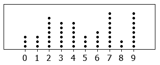
For smaller datasets, we can use an even simpler tally method. Dot plots represent the frequency of numerical or categorical data using individual dots stacked along an axis. If twelve students prefer band, you stack twelve dots above the "Band" label. It provides an immediate, tactile count of the data.

A dot plot stacks individual data points along a single axis, providing a direct visual tally of frequencies for small datasets.

Circle Graphs

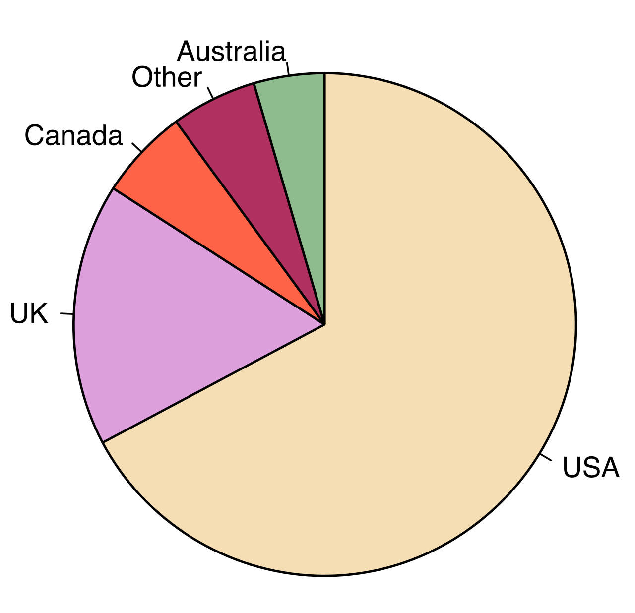
Sometimes, the absolute count matters less than the slice of the pie. Circle graphs display categorical data as proportional parts of a whole. They force the viewer to see the data as fractions of a single, unified population. Because it represents the entirety of a dataset, the sum of all percentage values in a complete circle graph is exactly 100 percent.

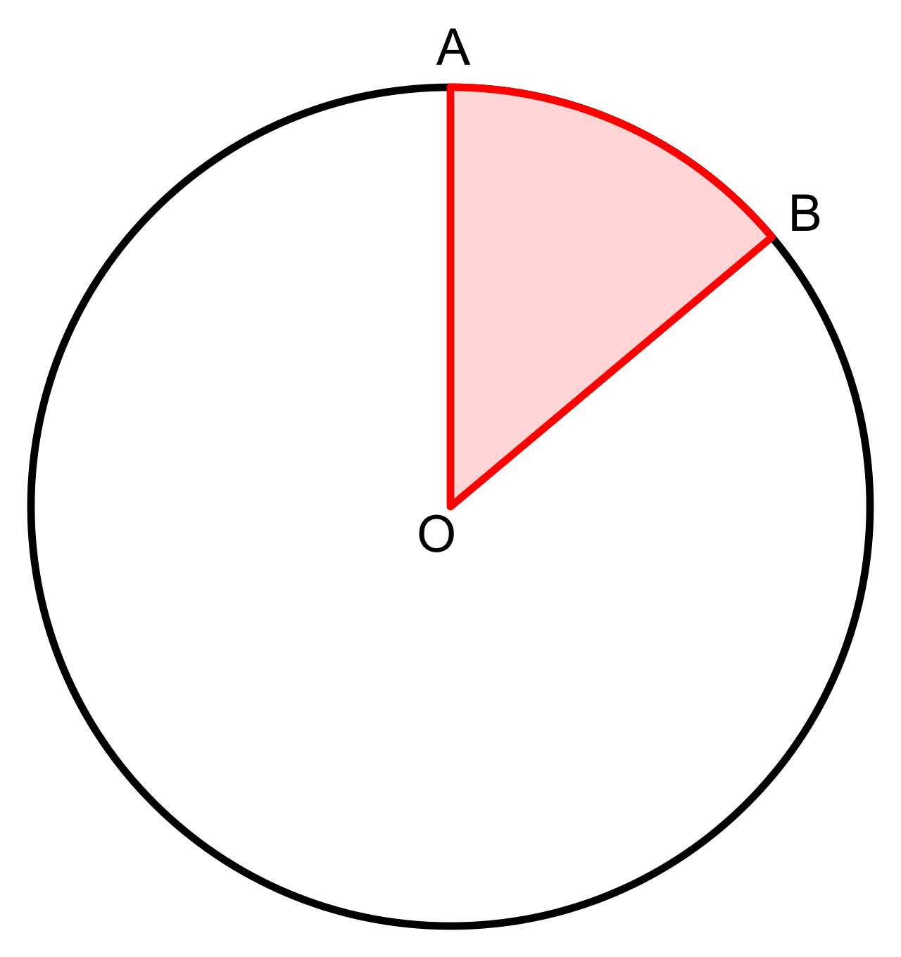
A circle graph, or pie chart, divides a population into proportional slices, with the entire circle representing exactly 100 percent of the dataset.

Constructing a circle graph is an exercise in geometric translation. The central angle of a sector in a circle graph is directly proportional to the relative frequency of that category. Since a full circle is $360^\circ$ , a category representing $25\%$ of the data must occupy a central angle of exactly $0.25 \times 360^\circ = 90^\circ$ .

The central angle of a sector is geometrically proportional to its relative frequency, calculated as a fraction of a full 360-degree circle.

When data is numerical, it naturally flows along a continuous number line. We are no longer looking at isolated buckets; we are looking at the shape, spread, and density of a distribution.

Preserving the Raw Data

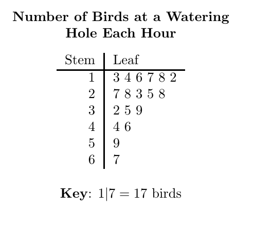
Sometimes, in the pursuit of visual summary, we do not want to lose the actual numbers. Stem-and-leaf plots display the frequency distribution of numerical data while preserving the exact original data values. If your students scored 82, 85, and 88, the "stem" is 8, and the "leaves" are 2, 5, and 8. You can see the bell curve taking shape, yet you can still extract every individual test score to calculate a precise mean.

A stem-and-leaf plot groups numerical data by place value, revealing the shape of the frequency distribution while preserving every exact data point.

Grouping the Data: Histograms

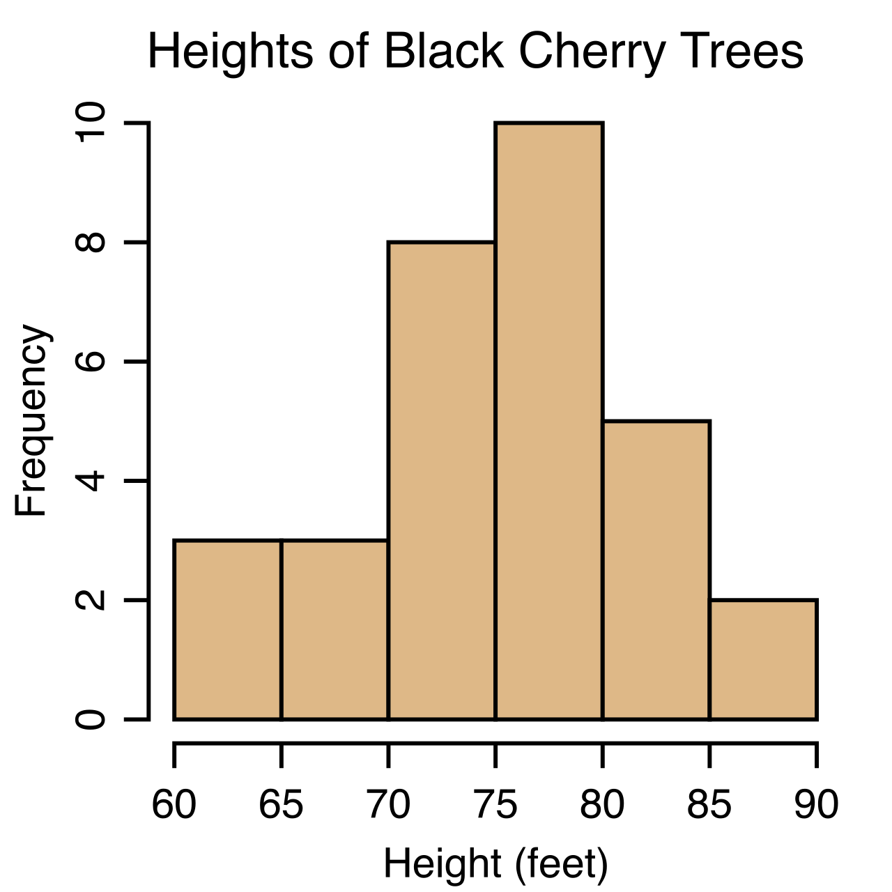
For larger continuous datasets—like the time it takes 200 students to complete a sprint—plotting every individual decimal value is chaotic. We must impose order. Histograms display the frequencies of continuous numerical data.

To build a histogram, the continuous number line is carved into segments. Data in a histogram is grouped into contiguous intervals called bins. Unlike the distinct bars of a categorical bar graph, a histogram has no spaces between its columns because the underlying data (e.g., time or distance) never stops flowing. A student could run a race in 15 seconds, 15.1 seconds, or 15.11 seconds.

To prevent visual manipulation, the bins in a histogram must be of equal width. If one bin spans ten seconds and another spans two, the visual representation of density collapses. In this structure, the height of a bin in a histogram represents the frequency of data values within that interval.

A histogram maps continuous numerical data into intervals or "bins" of equal width. The absence of gaps between columns reflects the continuous nature of the variable.

Summarizing Spread: Boxplots

Teachers frequently want to strip away the noise of a dataset and look purely at its structural center and extremes. Boxplots display the distribution of numerical data using a five-number summary.

The Five-Number Summary: The five-number summary for a boxplot consists of the minimum, first quartile, median, third quartile, and maximum.

This tool is a masterpiece of proportional design. The box in a boxplot spans from the first quartile ( $Q_1$ ) to the third quartile ( $Q_3$ ). The physical width of this rectangle is highly informative: the length of the box in a boxplot represents the interquartile range (IQR). By definition, the interquartile range contains the middle 50 percent of the numerical data values. If you want to know how your "typical" students performed, ignoring the handful who ace the test or completely bomb it, you look at the box.

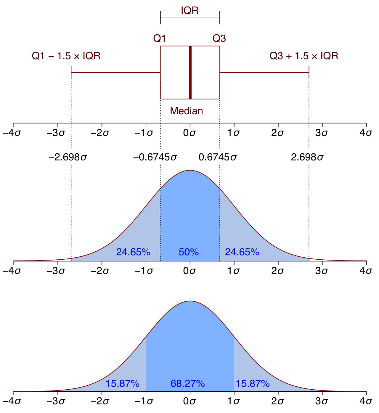
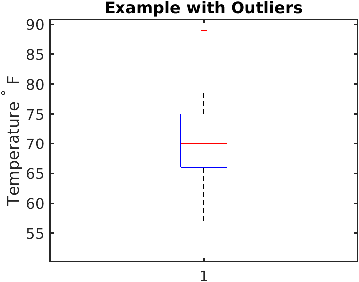
A boxplot summarizes a distribution by highlighting its median and quartiles. The central box aligns with the interquartile range, capturing the middle 50 percent of the data.

Reaching outward, the whiskers in a standard boxplot extend from the quartiles to the minimum and maximum values. However, nature is rarely perfectly tidy. When a data point is absurdly high or low compared to the rest of the distribution, drawing a massive whisker to reach it would distort our view of the typical spread. Therefore, outliers in a boxplot are often plotted as individual data points beyond the reach of the whiskers.

Extreme values, or outliers, are often plotted as isolated points beyond the whiskers to prevent them from exaggerating the visual spread of the typical data.

Often, we are not interested in a single variable, but in how two variables interact. Do students who study longer get higher scores? Does a heavier backpack correlate with a shorter vertical jump?

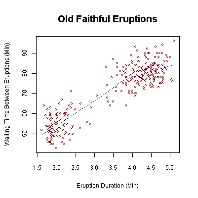
When both variables are continuous and numerical, we map them onto a Cartesian grid. Scatterplots display data points on a coordinate plane to model the relationship between two continuous numerical variables. Each point represents a single subject measured in two ways (e.g., $x =$ hours studied, $y =$ exam score).

If a pattern emerges from the cloud of points, we attempt to capture its essence. A trend line on a scatterplot models the general direction of the plotted data points. This line cuts through the center of the cloud, allowing us to make predictions about future behavior.

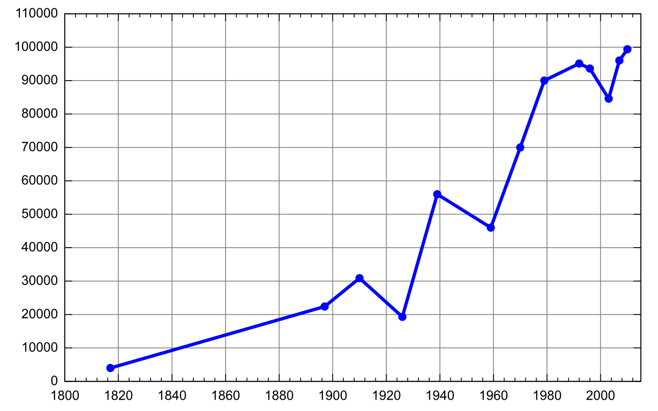
A scatterplot maps two continuous numerical variables on a Cartesian coordinate plane, making it easier to spot correlations, clusters, and overall trends.

When one of these continuous numerical variables is time, the dots are logically connected in sequence. Line graphs display continuous numerical data over a continuous variable such as time. Connecting the dots makes sense here because the time between Tuesday and Wednesday actually occurred, and the line implies the transition between the two measurements.

Line graphs connect sequential data points to model continuous changes, most commonly illustrating how a numerical variable shifts over time.

What if we want to find relationships, but our data is categorical, not numerical? You cannot plot "Choir" and "Soccer" on an $x,y$ coordinate plane. Instead, we use matrix formatting. Two-way tables summarize the frequencies of two categorical variables within a single dataset.

Imagine you survey 200 middle schoolers on two categorical variables: whether they are in the school band (Yes/No) and whether they are on the honor roll (Yes/No).

	Honor Roll (Yes)	Honor Roll (No)	Row Totals
Band (Yes)	40	10	50
Band (No)	60	90	150
Column Totals	100	100	200

Decoding the Frequencies

Every number in this table has a specific statistical identity.

Joint frequencies in a two-way table represent the count of data points belonging to a specific row category and a specific column category simultaneously. (e.g., The 40 students who are both in Band and on the Honor Roll).
Marginal frequencies in a two-way table represent the total sum of counts for a single row or a single column. These live in the margins of the table. (e.g., The 50 total students in Band, or the 100 total students on the Honor Roll).
The grand total in a two-way table is the sum of all joint frequencies. Here, the 200 surveyed students.

Establishing Proportions with Relative Frequencies

Raw counts can be deceiving. If 60 non-band members are on the honor roll, and only 40 band members are, does that mean avoiding band makes you a better student? Not necessarily. There are far more non-band members in total! To compare categories fairly, we must standardize the data.

Relative frequency is the ratio of a specific frequency to a designated total count. By dividing counts by totals, we create percentages (or decimals) that level the playing field.

A joint relative frequency is calculated by dividing a joint frequency by the grand total.
- Example: Band AND Honor Roll $\rightarrow \frac{40}{200} = 0.20$ (or $20\%$ ).
A marginal relative frequency is calculated by dividing a marginal frequency by the grand total.
- Example: Total students in Band $\rightarrow \frac{50}{200} = 0.25$ (or $25\%$ ).

But the most powerful tool for a teacher or researcher is the conditional relative frequency. It restricts the universe to just one specific group. A conditional relative frequency is calculated by dividing a joint frequency by a marginal frequency.

Let us ask a critical question: If a student is in the band, what is the probability they are on the honor roll? We ignore the grand total of 200. Our denominator becomes the 50 band members.

$\frac{40 \text{ (joint: Band and Honor Roll)}}{50 \text{ (marginal: Total in Band)}} = 0.80$ (or $80\%$ ).

Now, what if a student is NOT in the band?

$\frac{60 \text{ (joint: No Band and Honor Roll)}}{150 \text{ (marginal: Total Not in Band)}} = 0.40$ (or $40\%$ ).

Proving an Association

We have just found something remarkable in our data. Comparing conditional relative frequencies determines whether a statistical association exists between two categorical variables.

If the variables were totally independent—if band membership had nothing to do with academic performance—the conditional relative frequencies would be roughly equal. Honor roll rates would be identical whether you played the flute or not. But in statistics, an association exists between two categorical variables if the conditional relative frequencies differ significantly across categories.

Because $80\%$ of band members are on the honor roll, compared to only $40\%$ of non-band members, a strong association exists. Band membership and honor roll status are mathematically linked in this dataset.

As a mathematics teacher, this is the power of the discipline you will impart to your students. Statistics is not merely a collection of charts to be memorized; it is the definitive method for piercing through the noise of raw data to uncover the truth of how variables interact in the real world.