Counting Techniques and Sample Spaces
Not sure you’re ready?
Take the ~3-minute readiness diagnostic and see where you stand.
Consider a student standing in the school cafeteria line, faced with a rigid set of choices: three types of sandwiches, two types of fruit, and two types of milk. On the surface, it is merely a matter of picking lunch. Mathematically, it is a gateway into combinatorial logic, representing a universe of twelve distinct possibilities. As a mathematics educator, your objective is to teach students how to navigate, quantify, and visualize these possibilities without having to enumerate them exhaustively. The study of counting techniques and sample spaces is the study of structured choice. It transforms the overwhelming complexity of real-world variables—from scheduling classes to predicting genetic traits—into precise, calculable outcomes.
Before we can calculate the likelihood of anything happening, we must define the universe of everything that could happen. In mathematics, we demand absolute precision in our terminology, because these terms form the foundation of all probabilistic reasoning.
When we observe a process that generates uncertain results—like rolling a die or drawing a name from a hat—we are conducting a probability experiment. At the conclusion of this experiment, we arrive at an outcome, which is a single, specific result that occurs at the end of a probability experiment. If a student chooses a turkey sandwich, an apple, and chocolate milk, that distinct combination is exactly one outcome.
However, we rarely care about just one outcome in isolation. We need a map of the entire territory. This map is the sample space, defined as the complete mathematical set of all possible distinct outcomes of a probability experiment. If we toss a standard six-sided die, the sample space is {1,2,3,4,5,6}.
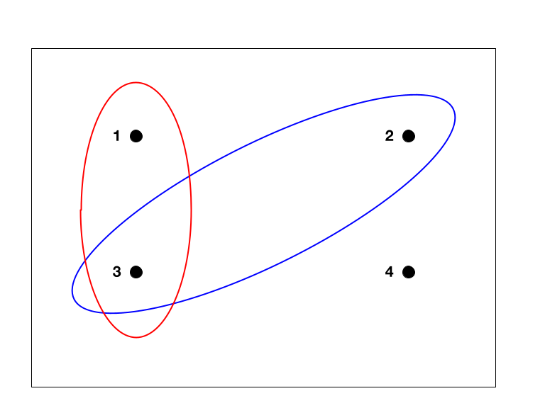
Often, we want to group certain outcomes together based on shared characteristics. An event is a defined subset of a sample space consisting of one or more outcomes. If our sample space is rolling a die, "rolling an even number" is an event consisting of the outcomes {2,4,6}.
Most real-world scenarios, however, do not involve just a single die roll or a single sandwich choice. A multi-stage probability experiment consists of two or more separate probabilistic events conducted sequentially or simultaneously. When a student chooses a sandwich, then a fruit, then a beverage, they are navigating a multi-stage experiment. To teach students how to handle this complexity, we must give them both visual tools and computational engines.
Human beings are visual creatures. When middle school students first encounter multi-stage experiments, asking them to calculate outcomes abstractly is a recipe for confusion. We must draw the map.
A tree diagram is a hierarchical graphical representation used to systematically map out all possible outcomes in a sequence of events. It breaks down the illusion of complexity into a series of simple, stepwise forks in the road.
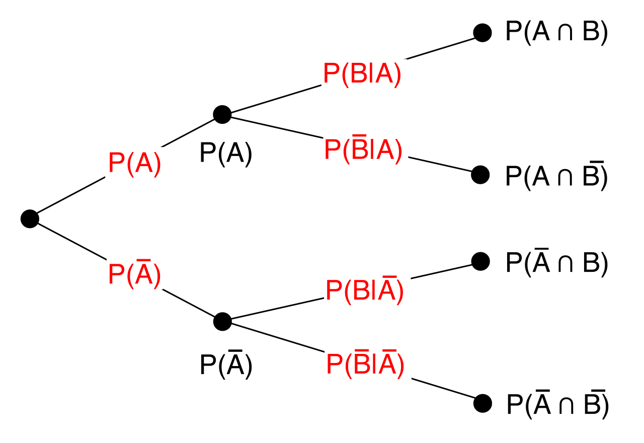
Here is the anatomy of a tree diagram:
- The Branches: In a tree diagram, each individual branch line represents one possible outcome of a single stage in an experiment.
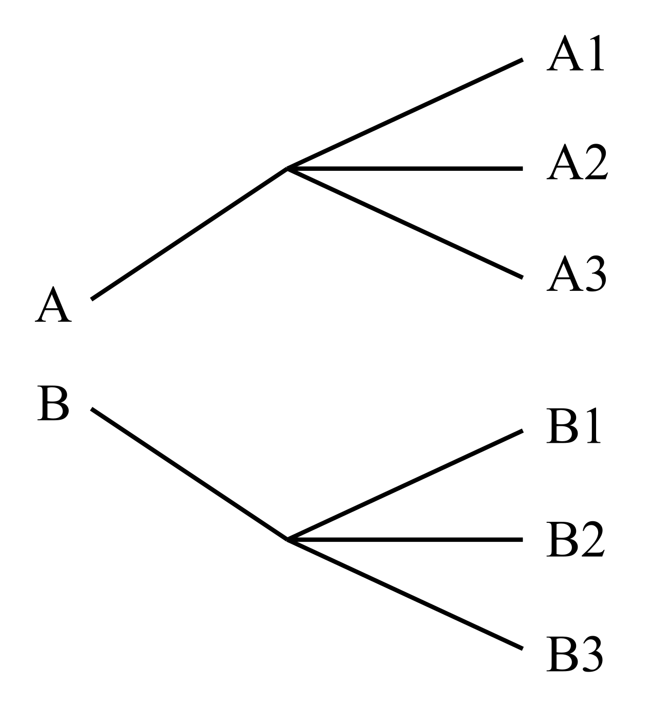
- The Progression: Constructing a tree diagram for consecutive events requires drawing a new complete set of branches originating from the endpoint of every branch of the preceding event. If Stage 1 has 3 branches, and Stage 2 has 2 options, you must draw those 2 options sprouting from the end of each of the 3 initial branches.
- The Path: Tracing a single continuous path from the starting root of a tree diagram to a final terminal branch identifies one specific, complete outcome of a multi-stage experiment.
- The Totality: The total number of terminal endpoints on the final branches of a completed tree diagram equals the total number of outcomes in the entire sample space.
By having your students physically trace a path with their fingers—from "Turkey" to "Apple" to "Chocolate Milk"—they internalize the concept that an "outcome" in a multi-stage experiment is a composite of several smaller choices. The terminal endpoints lay out the sample space perfectly before their eyes.
Tree diagrams are beautiful and conceptually vital, but they possess a fatal flaw: they do not scale. If a student needs to choose a 4-digit locker combination from a 40-number dial, drawing a tree diagram with 2,560,000 terminal endpoints is impossible. We must transition from visualization to algebraic calculation.
The Multiplication Rule
At the heart of combinatorics is a profound yet wonderfully simple axiom. The Fundamental Counting Principle states that if one event can occur in m ways and a second event can occur in n ways, the sequence of the two events can occur in m×n ways.
Because of this specific operation, the Fundamental Counting Principle is frequently referred to as the multiplication rule of counting in mathematics.
Furthermore, this is not limited to two events. The Fundamental Counting Principle extends to any number of sequential events by multiplying the number of possible outcomes for each individual event together.
The Fundamental Counting Principle (Multiplication Rule) Number of Outcomes = n1×n2×n3×⋯×nk
If our cafeteria has 3 sandwiches, 2 fruits, and 2 milks, the total number of lunch combinations is simply 3×2×2=12. The student arrives at the exact number of terminal endpoints on a tree diagram with a single line of arithmetic.
The Addition Principle
You must be exceptionally careful, however, to teach your students when to multiply and when to add.
The Addition Principle of counting states that if two events cannot happen at the same time (they are mutually exclusive), the total number of ways either event can occur is the sum of the number of ways each event can occur.
Think of it as the difference between "AND" and "OR".
- If a student must choose a sandwich AND a fruit, we multiply (m×n).
- If a student is told they can have EITHER a piece of fruit (2 choices) OR a dessert (3 choices), but not both, we add (2+3=5 choices total).
When extending the Fundamental Counting Principle to drawing items from a finite set—such as drawing marbles from a bag, or selecting students for a presentation order—the conditions of selection dramatically alter the mathematics. We must look at the population pool.
Sampling with replacement means a selected item is returned to the population pool before the next selection. Because the item goes back into the mix, sampling with replacement maintains a constant total number of choices for every subsequent event in an experiment.
- Example: Guessing a 4-digit PIN. You can use the digit '7' multiple times. The number of choices remains 10 for each digit: 10×10×10×10=10,000.
Conversely, sampling without replacement means a selected item is permanently removed from the population pool after selection. Consequently, sampling without replacement reduces the total number of available choices by exactly one for each subsequent selection step.
- Example: Selecting 4 different students to stand in a line. The first spot has 30 possible students. The second spot only has 29, the third 28, and the fourth 27. The calculation is 30×29×28×27.
Once students grasp sampling without replacement, they are ready to explore the most elegant counting techniques in algebra: permutations and combinations. Before we calculate them, we need a special notation to handle the cascading multiplication of "counting down."
Factorials: The Mechanics of Arrangement
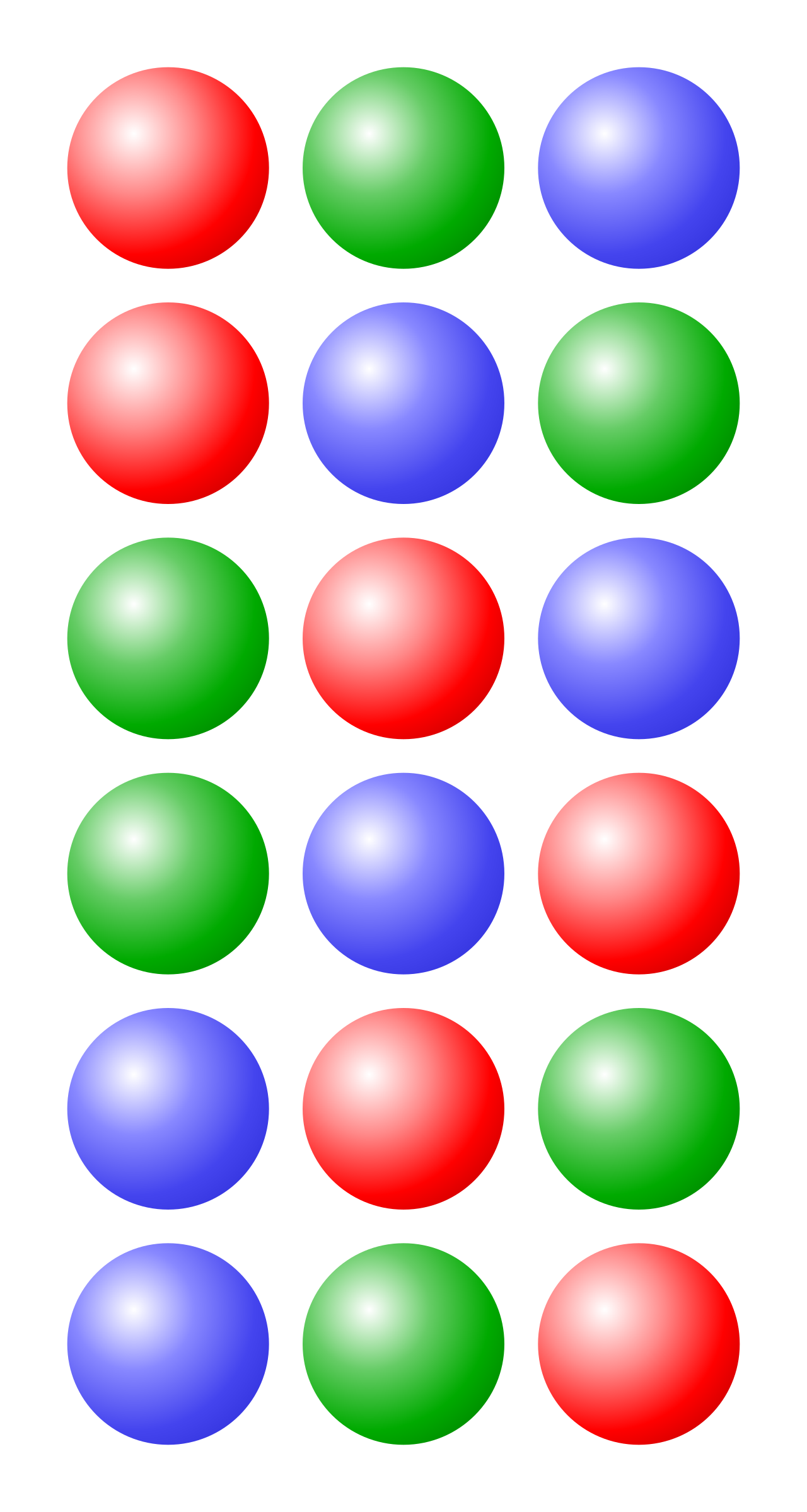
When we arrange n distinct items in a row, we are sampling without replacement until the pool is empty. For 5 books on a shelf, there are 5 choices for the first spot, 4 for the second, 3, 2, and 1 for the last.
This cascading multiplication is so fundamental to counting that it earns its own mathematical operator. The factorial of a positive integer n, written as n!, is the mathematical product of all positive integers less than or equal to n.
Factorial Definition: n!=n×(n−1)×(n−2)×⋯×3×2×1 Example: 5!=5×4×3×2×1=120
There is a vital edge case you must be prepared to explain: $0!$ (zero factorial) is defined by convention to be exactly 1. Why? Pedagogically, you can explain this intuitively: How many ways are there to arrange zero objects? There is exactly one way to do it—do nothing. Mathematically, it ensures that the formulas for permutations and combinations do not break by dividing by zero when selecting all or none of a set of items.
Permutations: When Order is Paramount
A permutation is an arrangement of a distinct set of objects into a sequence where the specific order of the objects matters.
Consider electing a Class President, Vice President, and Treasurer from a group of 20 students. Selecting Alice as President and Bob as VP is fundamentally different from selecting Bob as President and Alice as VP. The specific order dictates the roles.
If we used our Fundamental Counting Principle, we would say: $20 \times 19 \times 18$. The mathematical community uses factorials to create a generalized formula for this.
Permutation Formula: The formula for calculating the total number of permutations of n distinct objects taken r at a time is n! divided by (n−r)!.
P(n,r)=(n−r)!n!
Notice how elegant this is! To calculate $20 \times 19 \times 18, the formula writes out the entire sequence from 20 down to 1 (\20!), and then divides out the tail end we didn't use (\17!).The(n-r)!$ in the denominator acts as an algebraic pair of scissors, snipping off the unwanted multiplication.
Combinations: The Democracy of Sets
A combination is a mathematical selection of objects from a larger group where the specific order of the selected objects does not matter.
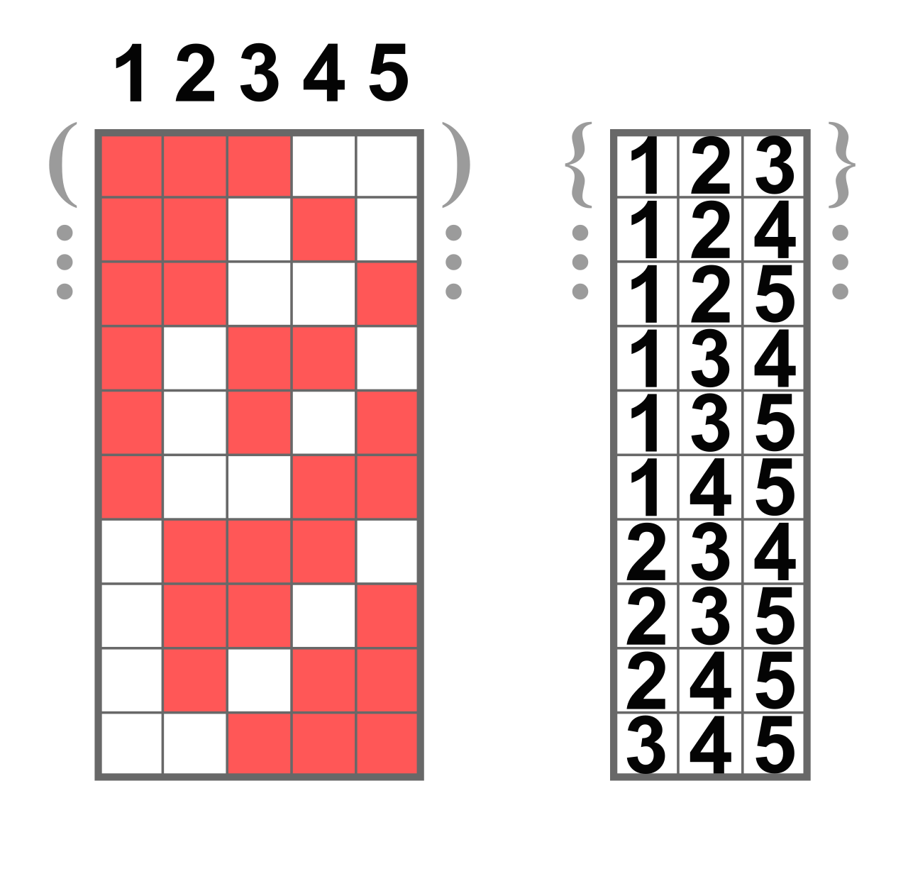
Consider choosing 3 students to form a cleanup committee from a group of 20. If I choose Alice, Bob, and Charlie, it is the exact same committee as choosing Charlie, Alice, and Bob. Order is utterly irrelevant.
If we blindly used the Permutation formula, we would calculate $20 \times 19 \times 18 = 6,840 arrangements. But we have severely overcounted! For every group of 3 students, we have counted them \3 \times 2 \times 1 = 6 times (which is \3!$, the number of ways to arrange 3 items).
To fix this overcounting, we must divide our permutation answer by the number of ways to arrange the selected items (r!).
Combination Formula: The formula for calculating the total number of combinations of n distinct objects taken r at a time is n! divided by the product of r! and (n−r)!.
C(n,r)=r!(n−r)!n!
Teacher's Guide: Permutation vs. Combination
On the Praxis 5164 exam, and in your future classroom, the hardest hurdle is not the arithmetic; it is the reading comprehension required to distinguish a permutation from a combination. Equip your students with this mindset:
| Characteristic | Permutations | Combinations |
|---|---|---|
| Defining Feature | Specific order matters. | Specific order does not matter. |
| Mental Trigger | Passwords, podium finishes (1st, 2nd, 3rd), distinct titles (President, VP), schedules. | Committees, a hand of cards, ingredients in a soup, drawing groups. |
| Formula | P(n,r)=(n−r)!n! | C(n,r)=r!(n−r)!n! |
| Outcome Quantity | Always yields a LARGER number than combinations for the same n and r (because rearrangements are counted separately). | Always yields a SMALLER number than permutations (because redundancies are divided out by r!). |
Mastering sample spaces and counting techniques isn't just about passing a licensure exam; it is about showing young learners how mathematics acts as a lens. It takes a chaotic world of infinite combinations—from the genetic lottery to the shuffling of a playlist—and demonstrates that with clear definitions, logical steps, and precise algebraic engines, the universe can be mapped, counted, and understood.