Statistical Processes and Sampling
Not sure you’re ready?
Take the ~3-minute readiness diagnostic and see where you stand.
Imagine trying to determine the average mathematics anxiety level of a middle school containing thousands of students. You could interview every single student, spending weeks disrupting classes and analyzing data, or you could carefully select a group of fifty and mathematically deduce the entire school's profile from their responses. The latter is the extraordinary power of statistical sampling. As a mathematics educator, you will not only use these tools to interpret your own classroom data, but you must also teach your students how to navigate a world overflowing with polls, studies, and statistical claims. To do this, we must rigorously understand how to ask the right questions, how to gather a mathematically sound sample, and the mechanisms of inference that allow us to generalize from the few to the many.
Mathematics is often taught as a discipline of absolute certainty—solve for x, and x is invariably 4. Statistics, however, is the mathematical discipline of measuring and taming uncertainty. This journey begins with how we frame our inquiries.
A statistical question is a question that anticipates variability in the data collected to answer the question. It expects that no single observation will tell the whole story.
Consider a simple statement: The question 'How old am I?' is not a statistical question because the answer does not vary. It is a single, deterministic fact. Conversely, the question 'How old are the students in my school?' is a statistical question because the ages of the students will vary.
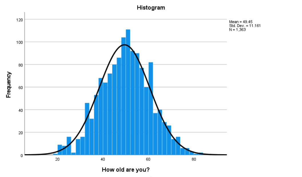
Because we anticipate variability, the data collected to answer a statistical question will not be a single number. Instead, the data collected to answer a statistical question will have a distribution with a center, spread, and overall shape. When you graph the ages of the students in your school, you might see a bell curve, a uniform block, or a skewed tail. Understanding statistics is about understanding the geometry of that distribution.
Before we measure anything, we must define the boundary of what we are measuring.
Population: The entire group of individuals or objects under study. Sample: A subset of individuals or objects selected from a population.
If you want to know the average height of every seventh grader in your state, the state's entire seventh-grade student body is your population. If you measure the heights of just your own seventh-grade class to guess the state average, your class is the sample.
Occasionally, researchers bypass sampling entirely. A census is a study that attempts to collect data from every individual in a population. While a census provides total certainty (eliminating the need to guess), it is often impractically expensive, time-consuming, or physically impossible. Therefore, we rely on samples. But not all samples are created equal.

If you want to know if a pot of soup is too salty, you don't need to drink the entire pot (a census); you just need a spoonful (a sample). However, if you haven't stirred the soup, and all the salt has sunk to the bottom, your spoonful will lie to you.
In statistics, an unstirred pot yields a biased sample, which systematically overrepresents or underrepresents certain segments of a population. Bias is not a matter of bad luck; it is a mechanical flaw in the sampling design itself.
There are two prevalent non-random sampling methods that reliably produce biased samples:
- Convenience Sampling: This is a non-random method where researchers select individuals who are easiest to reach. If you want to gauge middle schoolers' interest in a new after-school algebra club, and you only ask the students sitting in the front row of your honors math class, you are using convenience sampling. As a mathematical rule, convenience sampling typically leads to a biased sample because the easiest-to-reach group rarely reflects the diversity of the whole population.
- Voluntary Response Sampling: This is a non-random method where individuals choose themselves to participate in a study. Think of an online survey asking students to rate the cafeteria food. Voluntary response sampling typically overrepresents individuals with strong opinions—usually those who are exceptionally angry or exceptionally thrilled, entirely missing the indifferent majority.
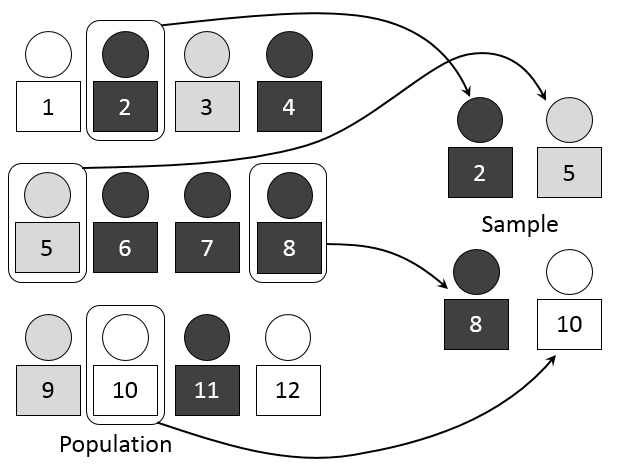
To avoid the unstirred pot, we must stir it. In statistics, "stirring" means introducing randomness. Random sampling uses a chance process to determine which members of a population are included in a sample. It removes human choice, convenience, and self-selection from the equation.
The most foundational method is the Simple Random Sample (SRS). For a sample to be a true SRS, two strict conditions must be met:
- Every individual in a population has an equal chance of being selected.
- Every possible group of a given size has an equal chance of being selected.
Imagine putting the names of all 500 students in your school into a giant hat and drawing 50 names blindfolded. Not only does student A have the exact same chance of being picked as student B, but the specific group of 50 students drawn has the exact same chance of being selected as any other combination of 50 students.
Advanced Random Sampling Techniques
While the SRS is conceptually perfect, it isn't always practical. Statisticians have developed advanced random sampling structures to ensure better representation across complex populations.
| Method | How It Works | The Middle School Analogy |
|---|---|---|
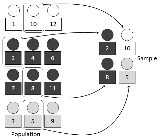
| Stratified Random Sampling | Involves dividing a population into homogeneous groups. Then, a simple random sample is drawn from each separate homogeneous group. | Divide the school into 6th, 7th, and 8th graders (homogeneous by age). Then, randomly select 20 students from each grade. |
| Cluster Sampling | Involves dividing a population into heterogeneous groups. Entire heterogeneous groups are randomly selected and all individuals within the selected groups are surveyed. | Treat each mixed-ability homeroom as a miniature version of the school (heterogeneous). Randomly pick three homerooms and survey every student inside them. |
| Systematic Random Sampling | Involves selecting every kth individual from a population list after a random starting point. | Get an alphabetical list of the whole school. Roll a die to pick a starting number (e.g., 4), then survey every 10th student after that (14th, 24th, 34th...). |
Even when you use a rigorous random sampling method, human behavior can still ruin your data. You must be able to recognize the mechanical failure points in data collection:
- Undercoverage bias occurs when the method of choosing a sample systematically excludes some part of a population. If you conduct a telephone survey of parents using a district landline directory, you systematically exclude families who only use cell phones or cannot afford a phone.
- Nonresponse bias occurs when selected individuals cannot be contacted or refuse to participate in a study. If you randomly select 100 students to take home a survey, but 40 of them leave it at the bottom of their backpacks and never return it, the missing 40 create nonresponse bias.
- Response bias occurs when the data collection method or question phrasing consistently produces misleading or untruthful answers. If a teacher stands in front of the class and asks for a show of hands to the question, "Have you ever cheated on one of my exams?", students will lie. The phrasing and environment induce response bias.
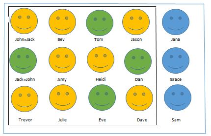
Why do we go through all this trouble to gather a random sample? We do it because we want to know a secret about the population, but we only have the resources to look at a sample. We need to define two critical terms that mirror each other:
Parameter: A numerical characteristic of an entire population. (Notice the mnemonic: Parameter describes the Population).
Statistic: A numerical characteristic calculated from a sample. (Statistic describes the Sample).
If the true average test score of all students in the district is 82%, that 82% is a parameter. It is the hidden truth. If you sample 40 students and find their average is 84%, that 84% is a statistic.
The heart of all statistics is bridging the gap between these two numbers. Statistical inference is the process of using data from a sample to draw conclusions about an entire population. In this process, a sample statistic serves as an estimate for an unknown population parameter.
Crucially, random sampling allows researchers to generalize conclusions from a sample to the broader population. If your sample is biased, inference is mathematically impossible. You cannot generalize from a convenience sample.
If you draw a random sample of 30 students and calculate their average height, and then I draw a different random sample of 30 students from the exact same school, we will likely get slightly different averages. This is not an error; it is sampling variability. Sampling variability is the phenomenon where different random samples of the same size from the same population produce different sample statistics.
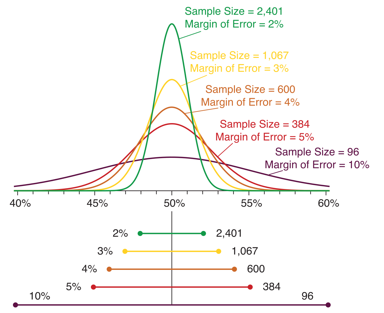
How do we tame sampling variability? We increase the size of our sample.
- Increasing the size of a random sample reduces the sampling variability.
- Because the variability shrinks, a larger random sample provides a more precise estimate of a population parameter than a smaller random sample.
However, there is a dangerous misconception that mere size fixes bad design. Increasing the sample size does not correct for sampling bias. If you are scooping soup from an unstirred pot where the salt is at the bottom, using a bigger spoon won't help you accurately estimate the saltiness of the top layer. You will just get a larger mouthful of incorrect data. Therefore, a large biased sample will consistently produce misleading conclusions about a population. A flawed sample of 10,000 is infinitely worse than a beautifully random, unbiased sample of 100.
Once we have our precise sample statistic, we want to know exactly how far off it might be from the true population parameter. We express this buffer zone using the margin of error.
The margin of error describes the expected maximum difference between a sample statistic and the true population parameter. If a poll says 60% of students want longer recess, with a margin of error of 3%, we infer the true population parameter likely rests somewhere between 57% and 63%. Because large samples are more stable, the margin of error decreases as the sample size increases.
Finally, we apply proportional reasoning, which scales up a sample proportion to predict outcomes for an entire population. Because a well-drawn random sample is mathematically representative of the whole, the ratios hold steady.
Therefore, if 20 percent of a random sample prefer a specific outcome, proportional reasoning predicts that 20 percent of the entire population prefers that outcome. If your school has 1,500 students, and your unbiased random sample reveals that 20% love algebra, you can confidently predict that roughly 300 students in the school (20% of 1,500) share that sentiment.
By mastering these concepts—identifying variability, eliminating bias, enforcing randomness, and applying proportional scaling—you transform raw data into a powerful lens. You move from guessing about your students to fundamentally understanding them.