Graphing Inequalities and Systems
Not sure you’re ready?
Take the ~3-minute readiness diagnostic and see where you stand.
When a school administrator decrees that a field trip requires at least one chaperone for every ten students, but the total bus capacity cannot exceed sixty passengers, they are not merely issuing logistical directives. They are defining a geometric space. Real-world limitations—budgets, time, physical space, and safety regulations—carve out boundaries in the Cartesian plane. Understanding how to graph and interpret systems of linear inequalities is the mathematical mechanism for finding the precise "zone of the possible" within these rigid constraints. As a mathematics educator, your objective is not just to teach students how to shade regions on a graph, but to show them how algebra translates the chaotic limits of the physical world into a visual map of viable solutions.
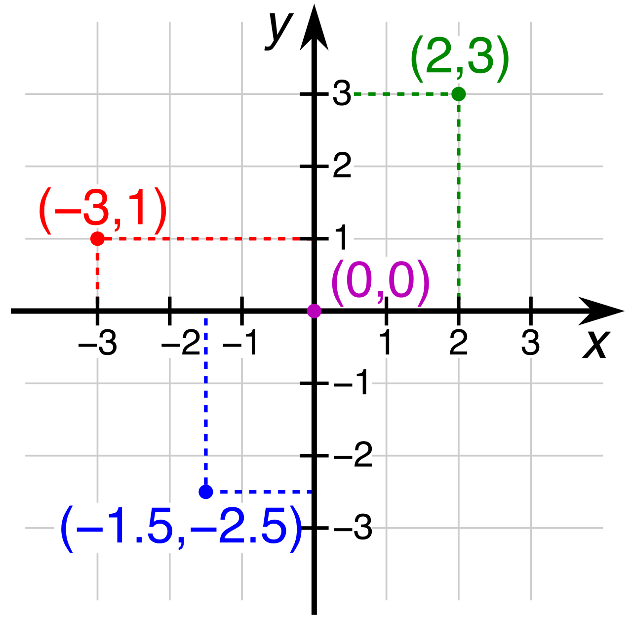
Every linear inequality begins with a conceptual line in the sand. When we graph an inequality, we first graph the corresponding equation. This line acts as a boundary line that completely divides the Cartesian coordinate plane into two distinct half-planes. One half-plane represents all the conditions where the inequality holds true; the other represents where it fails.
Drawing the Boundary
The physical appearance of the line tells us exactly how to treat the boundary itself:
- Solid boundary lines: A solid boundary line on a graph indicates that points lying directly on the line are included in the solution set of the linear inequality. We use a solid boundary line when representing a linear inequality utilizing the greater-than-or-equal-to symbol (≥) or the less-than-or-equal-to symbol (≤).
- Dashed boundary lines: Conversely, a dashed boundary line on a graph indicates that points lying directly on the line are explicitly excluded from the solution set of the linear inequality. We draw a dashed boundary line to represent a linear inequality utilizing the strict greater-than symbol (>) or the strict less-than symbol (<).
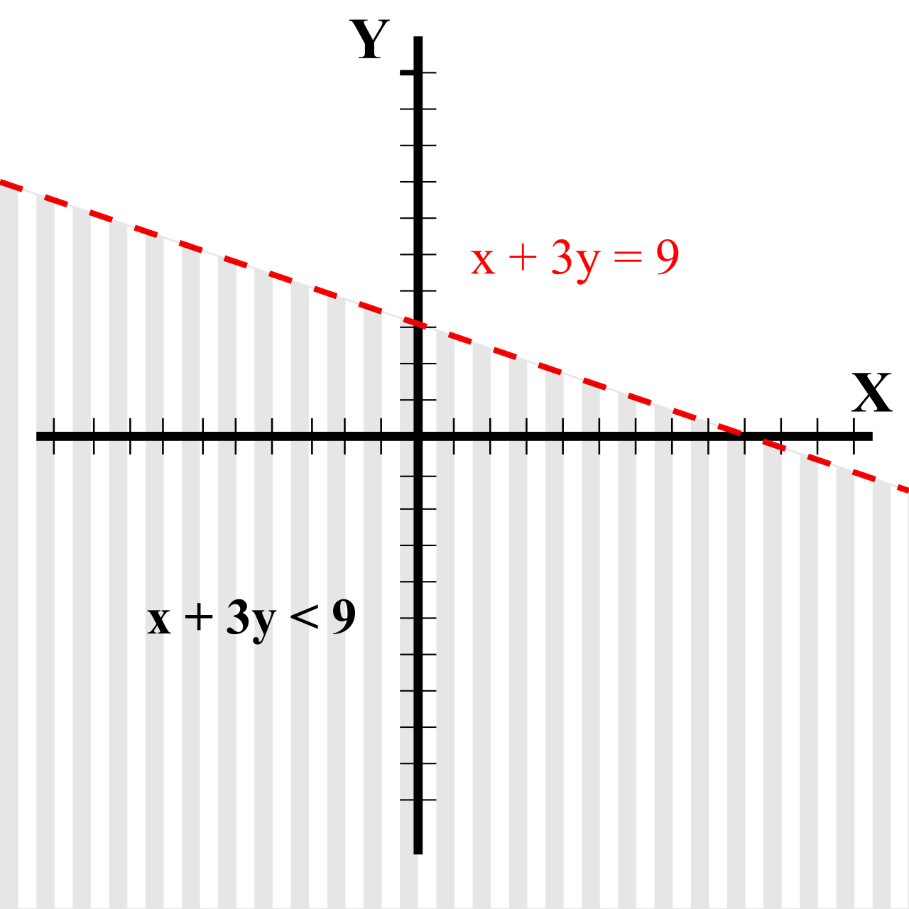
The Feynman Rule of Boundaries: Think of a solid line like a brick wall you can lean against—you are part of the structure. A dashed line is like an electric fence—you can get infinitely close to it, but you cannot actually touch it.
Finding the Solution Space
Once the boundary is established, we must determine which half-plane contains our solutions. There are two primary techniques for finding the correct region:
- The Test Point Method: A test point not located on the boundary line can determine which half-plane contains the solutions to a linear inequality. The origin (0,0) is the most efficient test point, provided the boundary line doesn't pass through it. Substituting a test point's coordinates into an inequality yields a true mathematical statement only if the test point lies in the solution half-plane. If the statement evaluates as true (e.g., 0<5), shade the half-plane containing the test point. If it evaluates as false, shade the opposite half-plane.
- The Vertical Alignment Method: If the inequality is solved for y (i.e., in slope-intercept form), the orientation is purely vertical. The region vertically above a non-vertical boundary line represents solutions to linear inequalities solved for y featuring a greater-than (>) or greater-than-or-equal-to (≥) symbol. Conversely, the region vertically below a non-vertical boundary line represents solutions to linear inequalities solved for y featuring a less-than (<) or less-than-or-equal-to (≤) symbol.
In the real world, we rarely face just one limitation at a time. We have a budget and a time limit. We need a minimum number of volunteers and a maximum number of supplies. When we graph these simultaneous rules, we create a system.
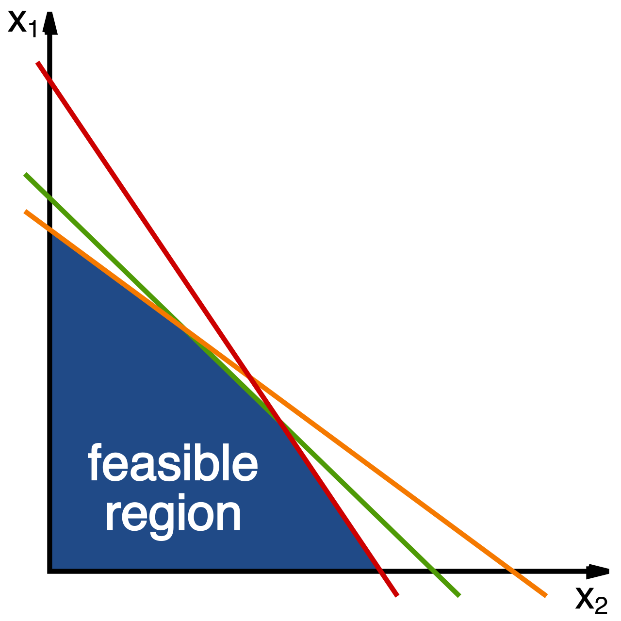
The solution set to a system of linear inequalities is the spatial intersection of the solution regions for each individual inequality within the system.
When graphing these systems on an on-screen calculator or by hand, the resulting overlapping shaded region is the heart of the matter. Any coordinate point located within the overlapping shaded region of a graphed system satisfies all individual inequalities in that system simultaneously.
Navigating the Edges of a System
The boundaries of this overlapping region require precise interpretation:
- Valid Edges: A point located on a solid boundary line of the overlapping intersection region is a valid solution to the overall system of linear inequalities.
- Invalid Edges: A point located on a dashed boundary line of the overlapping intersection region is not a valid solution to the overall system of linear inequalities.
- Vertices: What happens at the corners where lines cross? The intersection vertex of two solid boundary lines is fully included in the solution set of a system of linear inequalities. However, an intersection vertex involving at least one dashed boundary line is strictly excluded from the solution set of a system of linear inequalities. A corner must be entirely solid to be a valid solution.
The Shape of the Possible
The spatial intersection of inequalities can take several geometric forms:
| Region Type | Description | Real-World Implication |
|---|---|---|
| Bounded | A system of linear inequalities can have a solution set bounded on all sides creating a closed polygonal region on the coordinate plane. | Resources are strictly limited from all sides (e.g., minimums required, maximums enforced). There is a finite range of possibilities. |
| Unbounded | A system of linear inequalities can have a solution set that remains unbounded and extends infinitely in at least one direction on the coordinate plane. | One or more variables have no upper limit. (e.g., You must produce at least 100 units, but you can produce as many more as you want). |
| No Solution | A system of linear inequalities with parallel boundary lines shaded away from each other contains no overlapping region and therefore has no solution. | The constraints are logically contradictory. (e.g., You must buy more than 10 computers, but you are forbidden from buying more than 5). |
To successfully teach middle school mathematics, we must build a bridge between abstract algebra and the lived environment of our students. Real-world operational constraints can be translated algebraically into a system of mathematical equations and linear inequalities.
When reading word problems, certain phrases are direct translations into specific mathematical symbols:
- Maximum limit constraints in real-world scenarios are typically modeled algebraically using less-than-or-equal-to inequalities (≤). Phrases like "no more than," "at most," or "maximum capacity" indicate that the boundary itself is acceptable, but nothing beyond it.
- Minimum requirement constraints in real-world scenarios are typically modeled algebraically using greater-than-or-equal-to inequalities (≥). Phrases like "at least," "no fewer than," or "a minimum of" require this symbol.
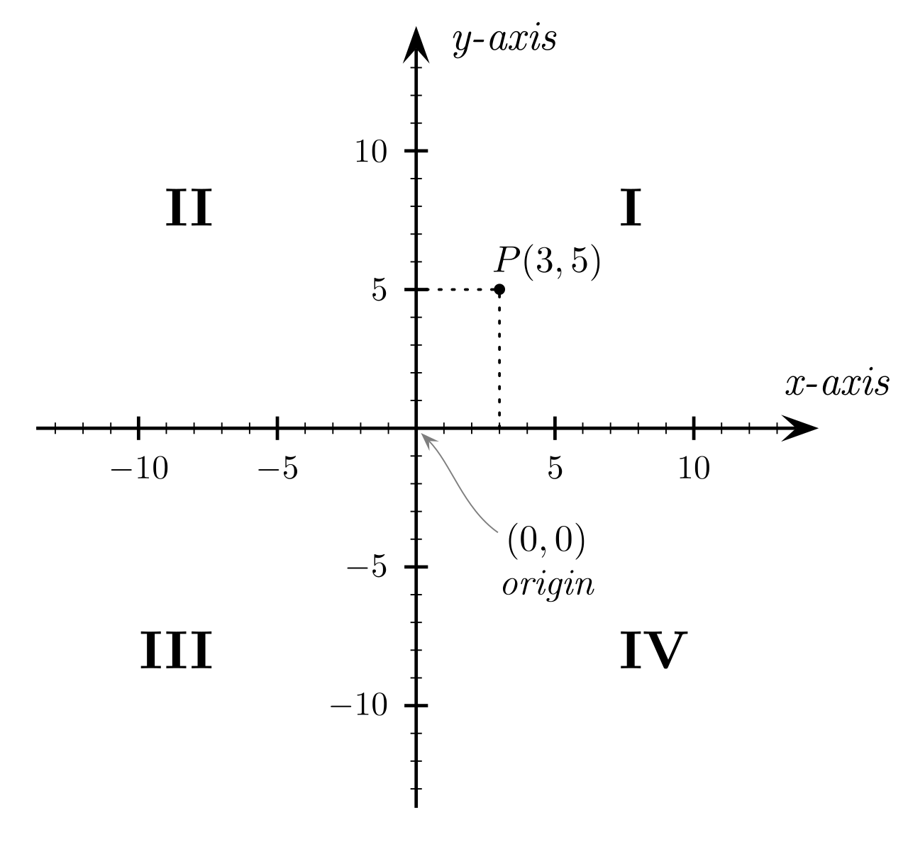
Furthermore, math in a vacuum allows variables to stretch infinitely into the negative numbers. But if x represents the number of pizzas ordered for a math club party, x=−3 is physically meaningless. Therefore, real-world contexts involving physical quantities often require non-negativity constraints restricting x to greater than or equal to zero (x≥0) and y to greater than or equal to zero (y≥0). Geometrically, these vital constraints confine our graphical search entirely to the first quadrant of the Cartesian plane.
This is where the true test of a student's mathematical maturity lies. It is not enough to find a point in the shaded region and declare victory. Viable solutions to applied problems must satisfy both the abstract mathematical system of inequalities and the logical limitations of the contextual scenario.
If a student uses a test point of (4.5,3.2) and it falls beautifully into the center of the shaded overlap, it mathematically satisfies the inequalities. However, a mathematically correct coordinate pair in an inequality solution set is considered nonviable if that pair violates the physical realities of the modeled word problem.
Discrete vs. Continuous Variables
The nature of what we are measuring dictates what solutions are physically viable.
- Discrete Variables: If a problem involves counting individual, indivisible units, we are dealing with discrete mathematics. Problems modeling discrete countable items strictly require whole number coordinates to be considered viable solutions. Consequently, fractional coordinate points located inside a mathematically correct shaded region are nonviable solutions when the variables represent discrete entities like human beings or cars. You cannot rent 2.5 buses, nor can you invite 14.7 students to a dance. Even if the point (14.7,2.5) is deeply nested inside the shaded region, it is entirely nonviable.
- Continuous Variables: Conversely, problems modeling continuous physical variables like time, distance, or fluid volume accept fractional and decimal coordinates as entirely viable solutions. If x represents hours spent driving and y represents gallons of fuel consumed, a coordinate pair of (3.5,8.25) is a perfectly logical, highly viable solution.
Teaching Takeaway for Praxis 5164: When interpreting items on the exam, always double-check the axes and variables. The exam will frequently test your ability to spot a point that is mathematically in the overlap but physically absurd. Remind your future students: Algebra gives us the map, but common sense tells us where we can actually stand.