Identifying and Evaluating Functions
Not sure you’re ready?
Take the ~3-minute readiness diagnostic and see where you stand.
A vending machine that unpredictably dispenses a water bottle on Tuesday and a bag of chips on Wednesday for the exact same button press is fundamentally broken. In mathematics, we demand predictability, which is why we distinguish between mere relations and functions. A mathematical relation is simply a set of ordered pairs mapping an input value to an output value—a historical record of what happened. But a function represents a strict mechanical guarantee: a specific type of mathematical relation where each input value maps to exactly one output value. As a future middle school educator, your task is to guide students from viewing mathematics as a loose collection of numbers to seeing it as the study of highly predictable systems. Grasping how to identify, evaluate, and classify these functional systems is the foundational step in that pedagogical journey.
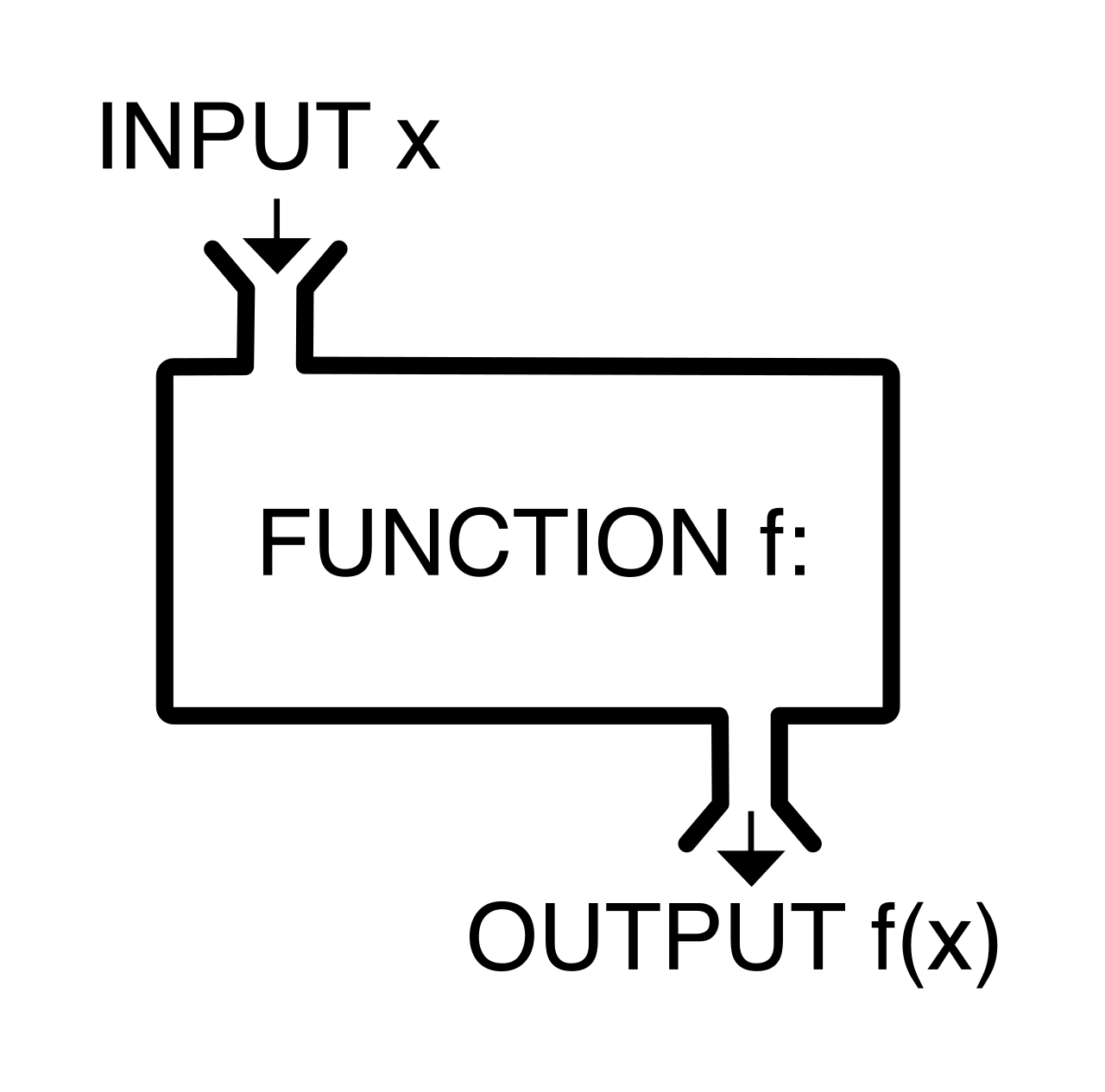
Every mechanical system operates within constraints: there are things you can put into it, and things it can produce. We formalize these constraints using domain and range.
The domain of a function is the complete set of all possible independent input values. The range of a function is the complete set of all possible dependent output values.
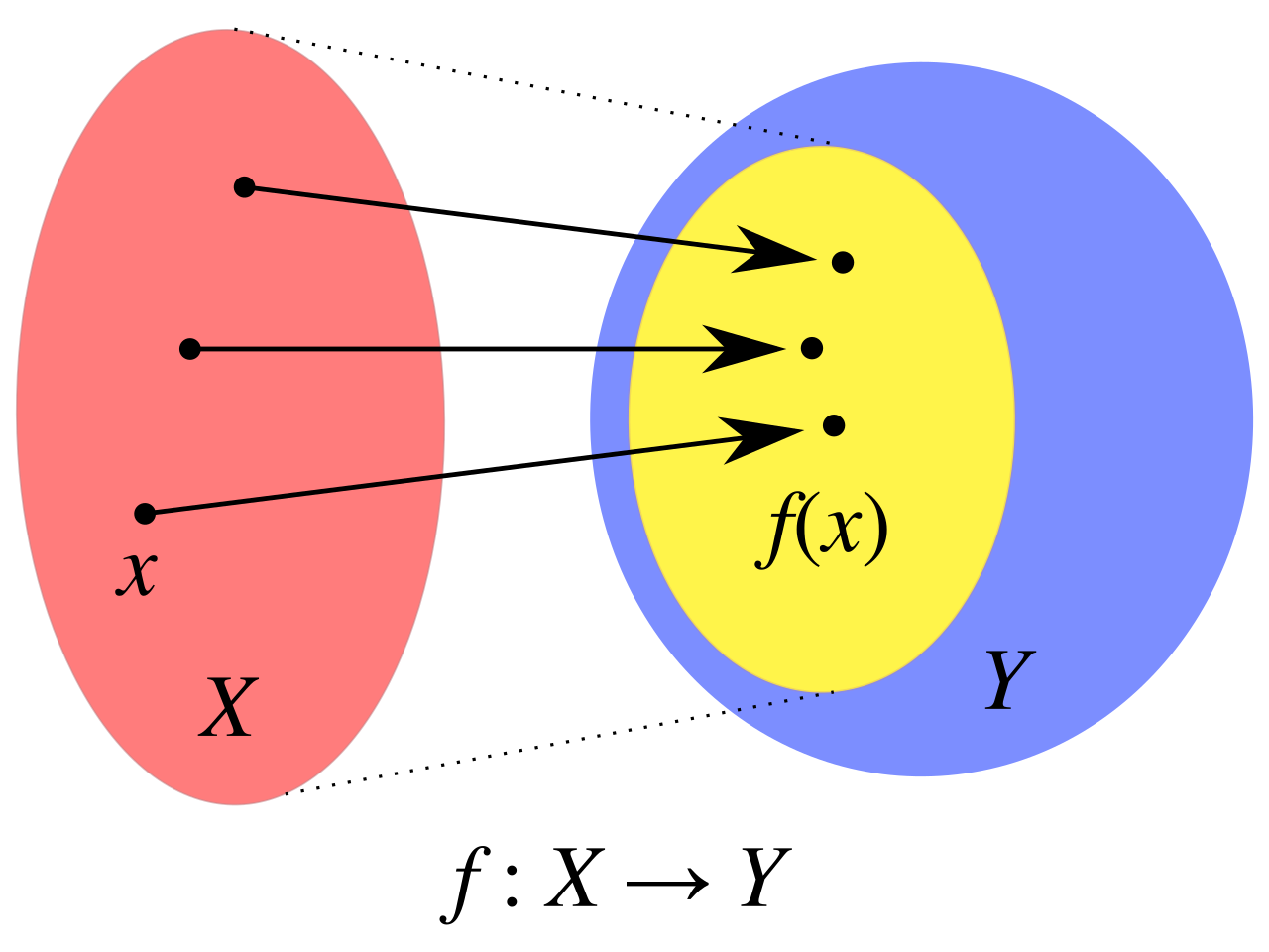
If the domain represents the buttons on our vending machine, the range represents the inventory inside. The critical rule of a function is that one button cannot yield two different types of items. This rule governs how we identify functions across various mathematical representations.
Identifying Functions from Data Sets
When looking at raw data, we are essentially looking for violations of our "broken machine" rule.
- Ordered Pairs: A set of ordered pairs represents a function if no two ordered pairs share the same first element with a different second element. The set {(2,5),(3,5)} is perfectly fine (two different buttons can dispense the same brand of water), but the set {(2,5),(2,9)} is a failure of the function rule.
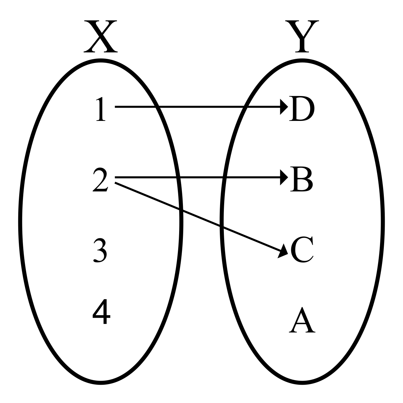
- Tables: Similarly, a table of values represents a function if no two distinct rows contain the same input value paired with different output values. As a teacher, you will often catch students scanning only the output column; remind them that repeated outputs are entirely legal. It is the inputs that must behave predictably.
The Algebraic Red Flags
When we define relationships algebraically, we use equations. However, not all equations are functions. The trap lies in operations that generate multiple answers for a single input.
An algebraic equation containing an output variable raised to an even power generally does not represent a function. Consider y2=x. If we input x=9, the output y could be 3, but it could also be −3. Because one input yielded two outputs, this is merely a relation.
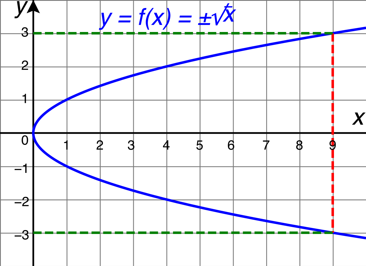
Similarly, an algebraic equation containing the absolute value of the output variable generally does not represent a function. In the equation ∣y∣=x, an input of x=5 forces y to split into 5 and −5. When teaching, point out that anytime the dependent variable (usually y) is hidden inside an even exponent or absolute value bars, the equation likely fails the definition of a function.
The Graphical Test
When we translate relations onto a coordinate plane, the test for predictability becomes beautifully visual.
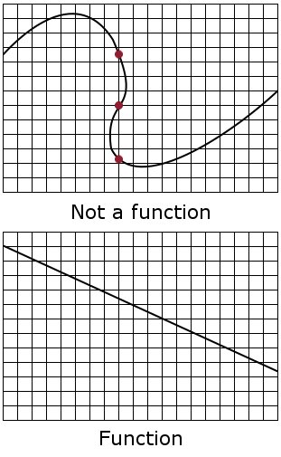
The vertical line test is a visual method used to determine if a graphical relation is a function. Because the horizontal x-axis represents the domain (inputs) and the vertical y-axis represents the range (outputs), a vertical line perfectly models a single input value.
Therefore, a graph represents a function if no vertical line drawn on the coordinate plane intersects the graph at more than one point. If a line slices through a curve twice, you have found an x-value mapped to two different y-values.
To communicate these mathematical systems clearly, we use function notation. In function notation, the symbol f(x) represents the output value of the function f for the specific input value x.
Evaluating a function simply means running the machine for a given input. We do this in three primary ways:
- Algebraically: Evaluating a function algebraically involves substituting a specific domain value for the independent variable in the function equation. If f(x)=3x+2, to evaluate f(4), we substitute 4 for x to get 14.
- Graphically: Evaluating a function from a graph requires finding the specified input value on the horizontal axis and identifying the corresponding output value on the vertical axis.
- Piecewise: Piecewise functions are composed of different algebraic rules for different parts of the domain. Evaluating a piecewise function requires identifying which domain interval contains the specified input value before substituting the input into the corresponding expression. Students intuitively try to plug the input into every piece; you must teach them that domain intervals act as routing systems, directing the input to one and only one equation.
In middle school mathematics, students explore a universe of functions, but three specific families form the cornerstone of algebraic thinking. Understanding their algebraic structures, graphical shapes, and tabular patterns is essential for any educator.
Linear Functions
Linear functions govern constant, steady growth—like earning a flat hourly wage.
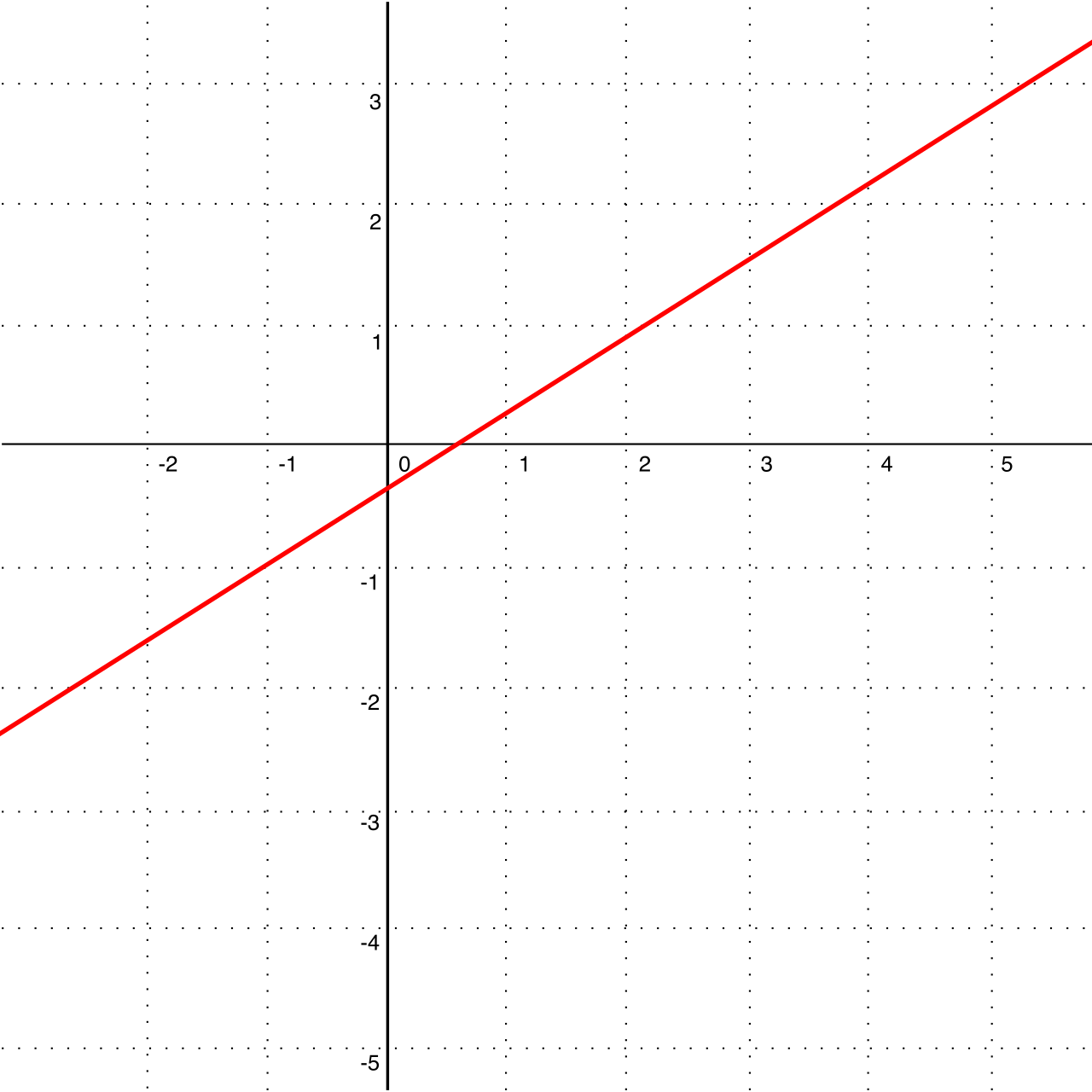
- Algebraic Form: A linear function is represented algebraically by an equation of the form f(x)=mx+b. The defining characteristic here is degree: the highest power of the independent variable in a linear function equation is exactly one.
- Graphical Form: Unsurprisingly, the graph of a linear function is a straight line.
- Tabular Pattern: To identify a linear function from a table, we examine the first difference of a mathematical relationship, which is the difference between consecutive output values for equal intervals of input values. A table of values represents a linear function if the first differences are a non-zero constant.
Quadratic Functions
Quadratic functions govern acceleration, gravity, and area. They represent growth that scales with itself.
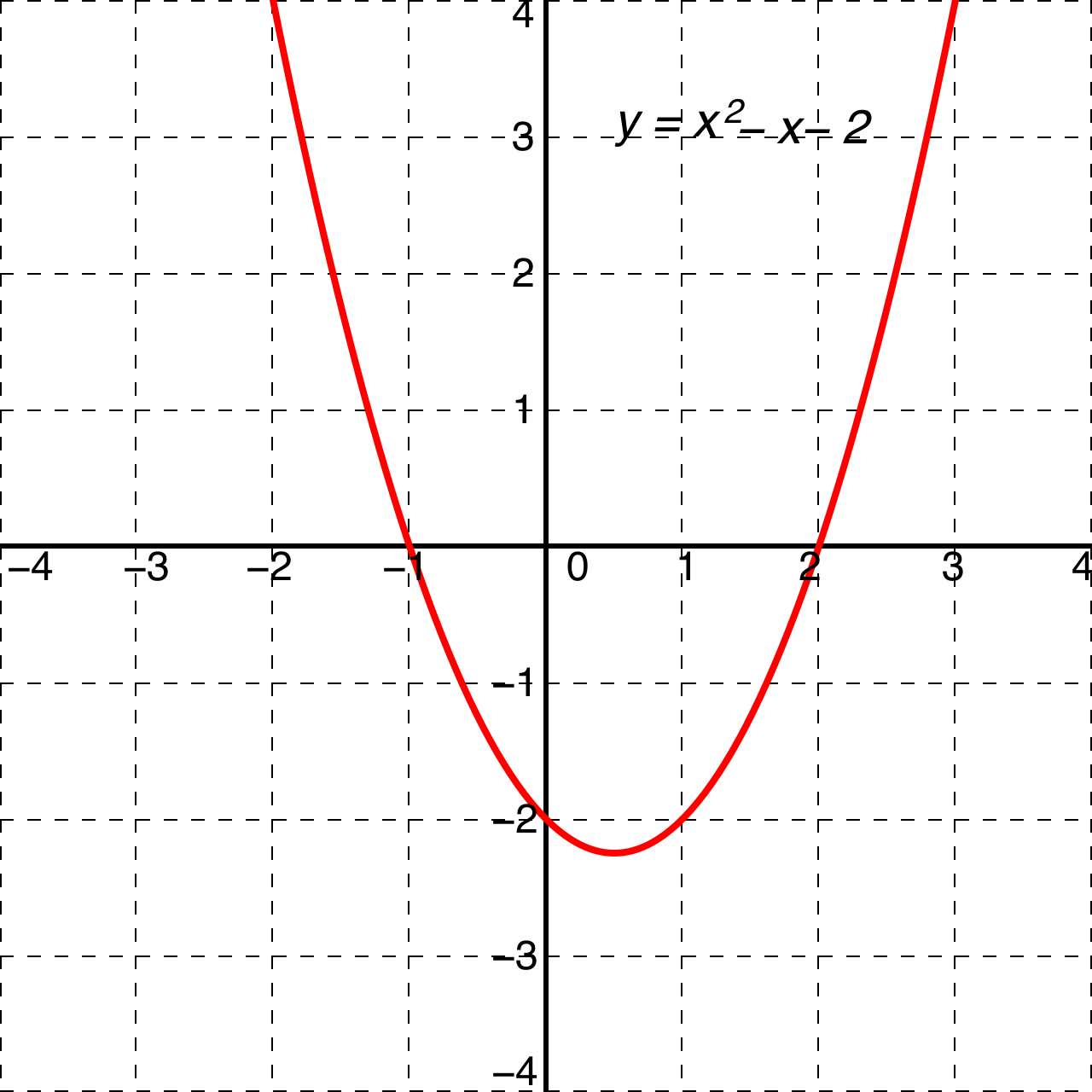
- Algebraic Form: A quadratic function is represented algebraically by a polynomial equation of degree two. The standard form of a quadratic function is f(x)=ax2+bx+c. To preserve that degree of two, there is a strict rule: the coefficient a must be a non-zero real number (if a=0, the x2 term vanishes, collapsing the function into a straight line).
- Graphical Form: The graph of a quadratic function is a U-shaped curve known as a parabola.
- Tabular Pattern: Because the growth rate of a quadratic is constantly changing, the first differences will not be constant. We must look deeper. The second difference of a mathematical relationship is the difference between consecutive first differences. A table of values represents a quadratic function if the second differences are a non-zero constant for equal intervals of input values.
Exponential Functions
Exponential functions model populations multiplying, viral spread, or compound interest. Here, the growth is multiplicative, not additive.
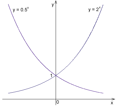
- Algebraic Form: An exponential function is represented algebraically by an equation where the independent variable appears as an exponent. The standard form of an exponential function is f(x)=abx.
- The Base Constraints: The base b behaves under strict mathematical laws to ensure the function remains continuous and predictable. In the equation f(x)=abx, the base b must be a strictly positive constant. (If b were negative, a fractional exponent like x=1/2 would force us to take the square root of a negative number, pulling us out of the real number system). Furthermore, the base b cannot equal one. If b=1, the function becomes f(x)=a(1)x, which flattens trivially into a horizontal line.
- Graphical Form: The graph of an exponential function sweeps upward or downward dramatically, but it also features a horizontal asymptote—a boundary line that the graph approaches infinitesimally closely without ever quite touching.
- Tabular Pattern: Because exponential functions grow by multiplication, we abandon differences and look at ratios. A table of values represents an exponential function if the ratio of consecutive output values is a constant factor for equal intervals of input values. This constant ratio of consecutive outputs directly represents the base multiplier of the exponential model (the b in f(x)=abx).
Summary of Tabular Identification
For quick recall during your exam, keep this matrix of tabular patterns in mind (assuming equal intervals of input values):
| Function Type | Algebraic Hallmark | Graphical Feature | Tabular Pattern (Equal Input Intervals) |
|---|---|---|---|
| Linear | Highest power is exactly 1 | Straight line | First differences are a non-zero constant |
| Quadratic | Degree 2 polynomial (a=0) | U-shaped parabola | Second differences are a non-zero constant |
| Exponential | Independent variable is exponent | Horizontal asymptote | Ratio of consecutive outputs is a constant factor |
By mastering the definitions, the constraints, and the core families of functions, you transition from someone who merely does math to someone who translates math. Whether evaluating f(3) on a piecewise graph or spotting the second difference in a quadratic table, these concepts form the rigorous, predictable engine underlying algebraic thought.