Systems of Linear Equations
Not sure you’re ready?
Take the ~3-minute readiness diagnostic and see where you stand.
A school district purchases a combination of 50 tablets and laptops for a new technology initiative. The total invoice arrives at $14,500. A tablet costs $200 and a laptop costs $450. Taken individually, these facts are merely constraints: one equation representing the total number of devices, and another representing the total budget. If we plot either constraint on a coordinate plane, we get an infinite continuum of possible scenarios. But when we impose both constraints on the universe at the same time, those infinite possibilities collapse into a single, unavoidable reality.
This is the essence of what mathematicians call a system of linear equations. Fundamentally, a system of linear equations consists of two or more linear equations containing the same variables. As a prospective middle school mathematics teacher, your task is to teach students how to navigate the transition between the physical reality of a problem, the algebraic manipulation of its symbols, and the geometric beauty of its graph.
Let us dissect the mechanics of these systems, how to solve them algebraically and graphically, and how these fundamental principles extend into the non-linear curves your students will encounter as they progress in their mathematical careers.
Before we manipulate a single algebraic symbol, we must establish what it actually means to "solve" a system.
The solution to a system of two linear equations in two variables is an ordered pair that satisfies both equations simultaneously.
Geometrically, graphing a system of linear equations reveals the solution as the coordinates of the intersection point of the lines. Every point on a line represents an ordered pair that makes that specific equation true. Therefore, the single point where two lines cross is the unique set of coordinates that makes both equations true at the same time.
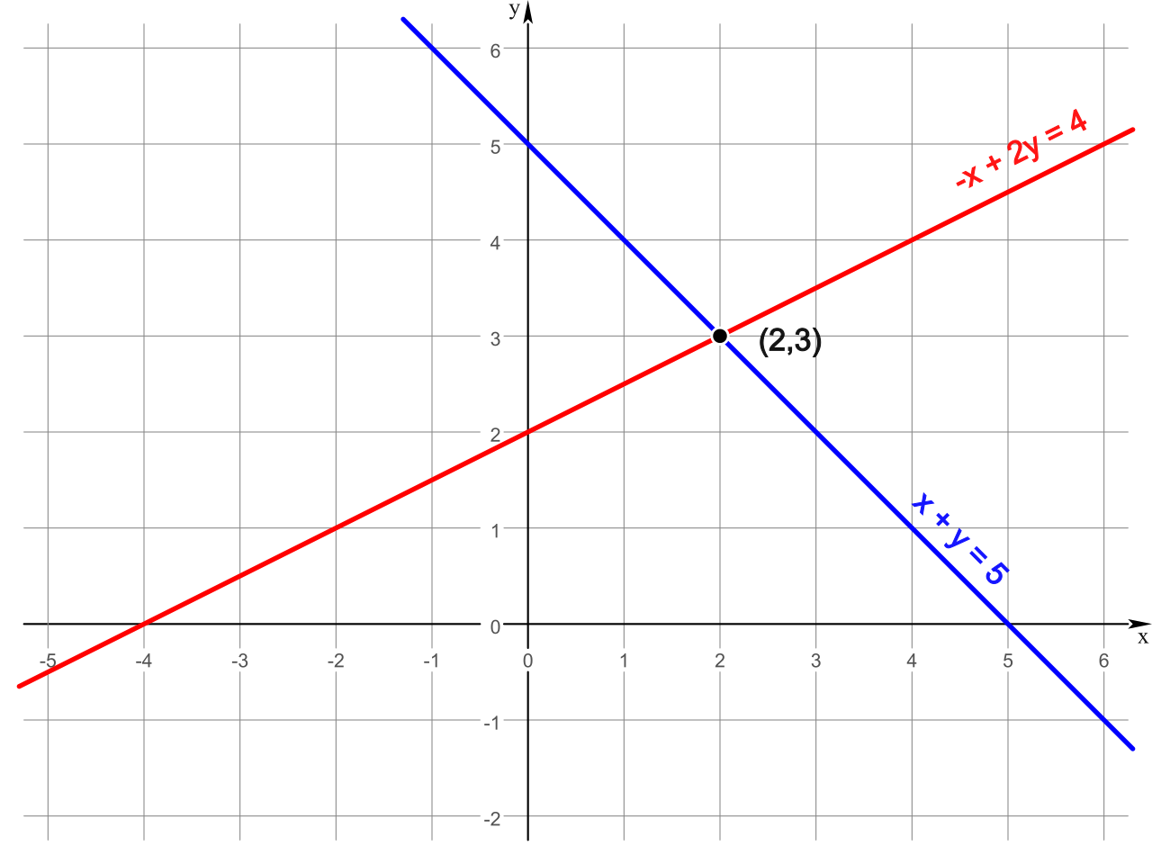
Crucially, you must impress upon your students the ultimate test of mathematical truth: verification. Any ordered pair calculated as a solution must yield a mathematically true statement when substituted back into every original equation within the given system. If it works in the first equation but fails in the second, it is not a solution to the system.
While graphing provides a beautiful visual intuition, algebra provides the precision required to find solutions without relying on perfectly drawn lines. We have two primary algebraic mechanisms to collapse a two-variable system into a solvable one-variable equation.
The Substitution Method
The substitution method relies on a simple premise: a variable is just a placeholder for a value. If we know exactly what an expression equals, we can swap it out.
The substitution method involves solving one equation for a single variable to isolate that specific variable. Once isolated, the expression for one variable replaces that exact variable in the second equation.
Imagine a system:
- y=2x+3
- 4x+y=15
Because the first equation explicitly tells us that y is entirely equivalent to the expression 2x+3, we drop that expression into the y-shaped void of the second equation, yielding 4x+(2x+3)=15. We have successfully bypassed the two-variable problem, reducing it to a single variable that a middle schooler can solve.
The Elimination Method
Sometimes, isolating a variable introduces messy fractions that obscure the logic of the math. In these cases, we turn to the elimination method—also commonly known as the addition method or the linear combination method.
The elimination method requires adding or subtracting the equations to completely remove one variable from the resulting equation. This works because if A=B and C=D, then A+C logically must equal B+D.
Often, equations are not perfectly primed for elimination. To use the elimination method, one or both equations might need multiplication by a constant to create opposite coefficients for a target variable.
Why are we allowed to just multiply an entire equation by an arbitrary number? Because of a beautiful geometric truth: multiplying an entire linear equation by a non-zero constant produces an equivalent equation with the exact same graphical line. If you scale 2x+3y=6 by a factor of 5 to get 10x+15y=30, you have not changed the fundamental relationship between x and y. You have simply rewritten the recipe. Once the coefficients of one variable are opposites (e.g., 3y and −3y), adding the equations vertically causes that variable to vanish, leaving a simple one-variable equation behind.
Not every system behaves identically. The relationship between the two lines dictates the number of solutions, and mathematics provides a precise vocabulary to classify these systems based on their geometry and algebraic behavior.
A system of equations with at least one valid solution is called a consistent system. If a system has no possible solutions, it is called an inconsistent system. Let us explore the three distinct archetypes.
1. Intersecting Lines (Exactly One Solution)
- Geometry: Two intersecting lines represent a system of linear equations with exactly one unique solution.
- System Type: Because it has exactly one single solution, it is an independent system (which is a subcategory of a consistent system).
- Structural Cause: A system of two linear equations with exactly one unique solution has equations with mathematically different slopes. If the slopes are different, the lines are guaranteed to cross exactly once in the Euclidean plane.
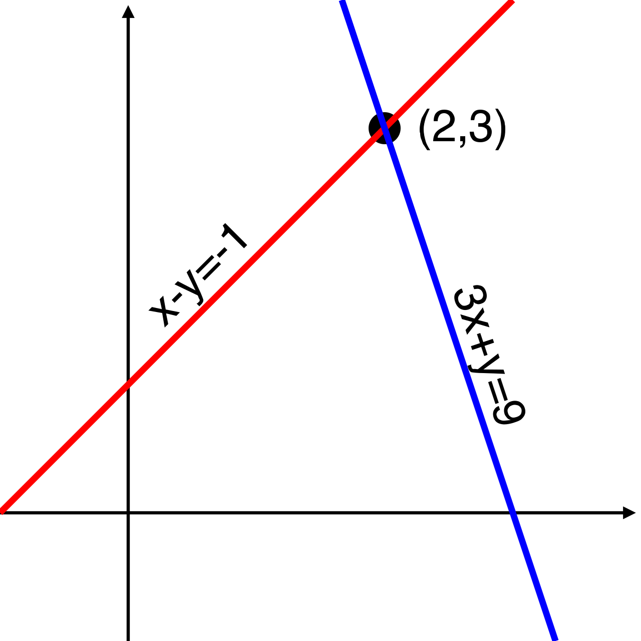
2. Parallel Lines (No Solution)
- Geometry: Two parallel lines represent a system of linear equations with absolutely no solution. They run infinitely alongside one another but never touch.
- System Type: Because there is no solution, this is an inconsistent system.
- Structural Cause: A system of two linear equations with no solution has equations with identical slopes and different y-intercepts. They have the same rate of change, but start at different places.
- Algebraic Signature: When you attempt to solve an inconsistent system algebraically, the variables will completely cancel out and leave a definitively false statement like 0=5 or 12=−4. This absurdity is algebra's way of telling you, "This scenario is physically impossible."
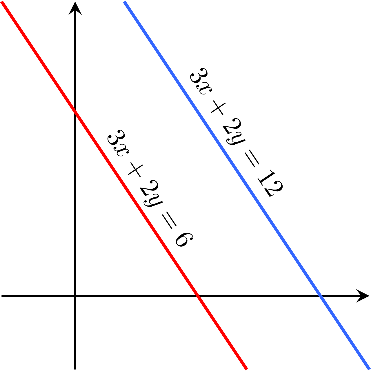
3. Coincident Lines (Infinitely Many Solutions)
- Geometry: Two coincident lines represent a system of linear equations with infinitely many solutions. Geometrically, they are the exact same line drawn on top of itself. Every point on the line is an intersection point.
- System Type: A consistent system of linear equations with infinitely many solutions is called a dependent system.
- Structural Cause: A system of two linear equations with infinitely many solutions has equations with identical slopes and identical y-intercepts.
- Algebraic Signature: Solving a system algebraically where the variables cancel out and leave a definitively true statement like 0=0 indicates infinitely many solutions. Algebra is confirming, "This statement is a tautology; it is true regardless of the values of x and y."
Summary Table for the Aspiring Teacher
| Geometry | Slopes & y-intercepts | Number of Solutions | System Classification | Algebraic Result |
|---|---|---|---|---|
| Intersecting | Different slopes | Exactly One | Consistent / Independent | x=a,y=b |
| Parallel | Same slope, different y-int | Zero | Inconsistent | False (e.g., 0=5) |
| Coincident | Same slope, same y-int | Infinitely Many | Consistent / Dependent | True (e.g., 0=0) |
As students transition toward advanced algebra, the concept of a system expands. The logic of intersection remains completely intact, but the geometry becomes richer.
Linear and Quadratic Systems
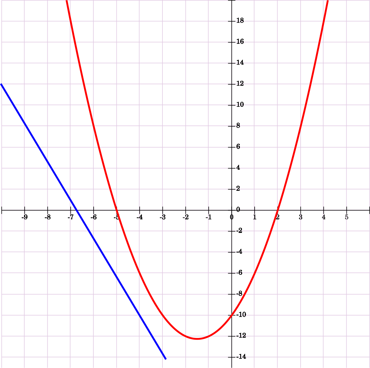
Imagine a flat plane intersected by a U-shaped parabola. The solution to a system containing a linear function and a quadratic function is the set of coordinate points where the line and the parabola intersect.
Because of the curvature of the parabola, a system consisting of one linear equation and one quadratic equation can have zero, one, or two real solutions.
- Two Solutions: The line slices through the interior of the parabola, crossing it at two distinct points (a secant line).
- One Solution: The straight line just barely grazes the outer edge of the parabola. A straight line that intersects a parabola at exactly one unique point is tangent to that parabola.
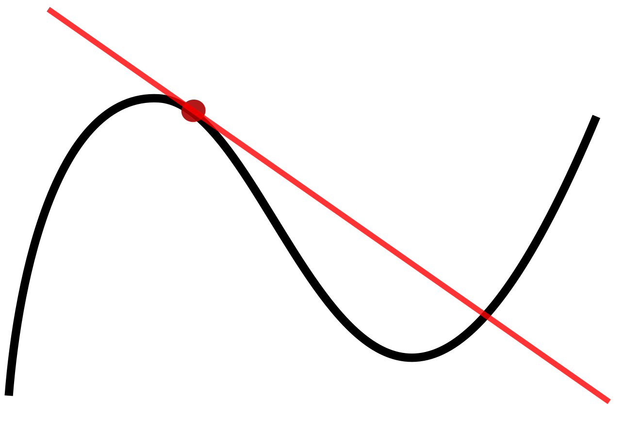
- Zero Solutions: The line misses the parabola entirely.
Linear and Exponential Systems
The principle holds for exponential growth and decay. The solution to a system containing a linear function and an exponential function is the set of intersection points of the straight line and the exponential curve.
Just like quadratics, a system consisting of one linear equation and one exponential equation can have zero, one, or two real solutions. Because an exponential curve bends dramatically (often accelerating rapidly away from a linear slope), it is entirely possible for a line to slice through it twice, graze it once, or miss it completely.
When dealing with messy coefficients or complex non-linear intersections, algebraic manipulation can become arduous or impossible for middle school students. This is where on-screen graphing calculators become invaluable pedagogical tools.
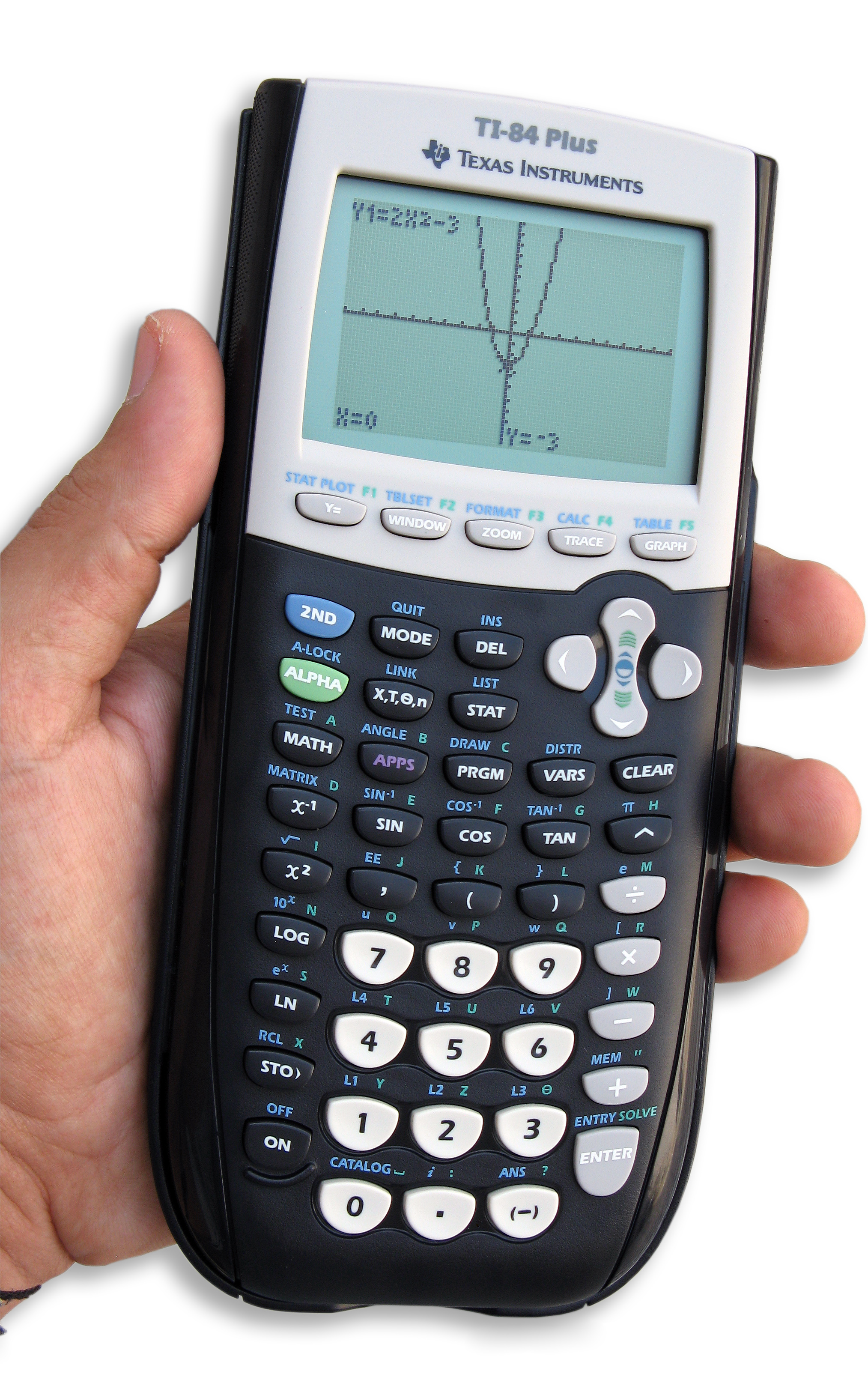
Graphing calculators provide approximate solutions to complex non-linear systems by calculating the coordinates of the intersection points visually or numerically.
If you want to find the exact x-coordinates of the intersection points of two functions f(x) and g(x), a student can graph both functions and find the specific x-values where f(x) equals g(x). Most graphing utilities have an explicit "intersect" command that computationally zeroes in on these coordinates.
Furthermore, we do not only have to rely on graphs. An approximate numerical solution to a system of equations can be found by creating tables of values for both functions and identifying where the output values are nearly equal. If f(3)=10.1 and g(3)=9.9, the student knows an intersection point exists incredibly close to x=3. This tabular method bridges the gap between pure algebra and pure geometry, building deep number sense.
Final Thoughts for the Praxis 5164
When you face the Middle School Mathematics exam, remember that a system of equations is a story told from multiple perspectives. Your mastery lies not just in solving x and y, but in knowing why the elimination method works, what a false algebraic statement signifies geometrically, and how to leverage technology to map out the exact points where vastly different mathematical functions collide. Lead your future students through this terrain, and they will see that algebra is not an arbitrary set of rules, but the precise language of logic and reality.