Solving Linear Equations and Inequalities

Not sure you’re ready?

Take the ~3-minute readiness diagnostic and see where you stand.

Imagine a precisely tuned mechanical scale resting on a laboratory bench, entirely level. The physical equilibrium of that scale is the tangible embodiment of mathematical equality. When we solve a linear equation, we are not simply executing a sequence of arbitrary algorithms; we are performing a carefully choreographed manipulation of weights that keeps the scale perfectly balanced from start to finish. For an aspiring middle school mathematics educator, mastering this choreography is not just about finding $x$ . It is about understanding the logical bedrock that allows us to manipulate mathematical reality without breaking it. When you teach these properties, you are giving your students the fundamental laws of a mathematical universe.

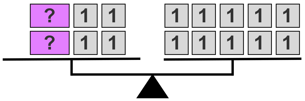
A simple balance scale serves as a powerful visual metaphor for algebraic equations, where operations must be applied equally to both sides to maintain mathematical equilibrium.

Before we manipulate algebraic expressions, we must establish the foundational rules of equality itself. When a middle school student solves $3x + 2 = 17$ and ends up with $5 = x$ , they often feel an instinctual need to rewrite it as $x = 5$ . As their teacher, you must explain why that is mathematically permissible.

The first recorded use of the equals sign by Robert Recorde in 1557, establishing the foundational visual symbol for representing mathematical equivalence.

The structure of equations is governed by four fundamental axioms:

The Reflexive Property of Equality: Any real number or mathematical expression is always equal to itself. Simply put, $x = x$ or $42 = 42$ . It is the most basic statement of identity.
The Symmetric Property of Equality: The left and right sides of an equation can be completely swapped without altering the truth value of the equation. If $a = b$ , then $b = a$ . This justifies the student rewriting $5 = x$ as $x = 5$ .
The Transitive Property of Equality: If a first quantity equals a second quantity, and the second quantity equals a third quantity, then the first quantity equals the third quantity. If $a = b$ and $b = c$ , then $a = c$ . This is the logical engine behind many algebraic proofs and geometric derivations.
The Substitution Property of Equality: If two quantities are equal, one quantity can replace the other in any algebraic expression without changing the value.

Verifying Solutions: The Substitution Property is practically applied when we check our work. Verifying a solution to a linear equation requires substituting the proposed numerical value back into the original equation to confirm it yields a mathematically true statement. If a student believes $x = 4$ is the solution to $2x = 8$ , substituting $4$ for $x$ yields $2(4) = 8$ , which is demonstrably true.

To isolate a variable, we must systematically dismantle the operations surrounding it while maintaining the equation's balance. We achieve this using four operational properties:

The Addition Property of Equality: Adding the same number to both sides of an equation maintains the equality of the two sides.
The Subtraction Property of Equality: Subtracting the same number from both sides of an equation maintains the equality of the two sides.
The Multiplication Property of Equality: Multiplying both sides of an equation by the same non-zero number maintains the equality of the two sides.
The Division Property of Equality: Dividing both sides of an equation by the same non-zero number maintains the equality of the two sides.

The Mechanics of Simplification

Often, an equation is too messy to solve immediately. Before shifting weights across the balance scale, we must consolidate the weights on each side.

Consider like terms: algebraic terms that contain the exact same variables raised to the exact same exponents. For instance, $4x$ and $7x$ are like terms, but $4x$ and $7y$ , or $4x$ and $7x^2$ , are not.

When your students simplify $4x + 7x$ to $11x$ , they are combining like terms. While this feels like simple addition, combining like terms is an algebraic simplification step formally justified by the Distributive Property.

The Distributive Property allows multiplying a single term across multiple terms grouped inside parentheses, represented as $a(b+c) = ab + ac$ . When read in reverse (factoring), it explains exactly why we can combine like terms: $4x + 7x = (4 + 7)x = 11x$ .

When your students apply these properties, they are embarking on an algebraic journey that leads to one of three distinct destinations.

1. One Solution The most common outcome occurs when a one-variable linear equation has exactly one solution if algebraic simplification isolates the variable to a single distinct value (e.g., $x = 5$ ). Geometrically, if you graphed the left side of the equation and the right side of the equation as independent lines, they would intersect at exactly one point.

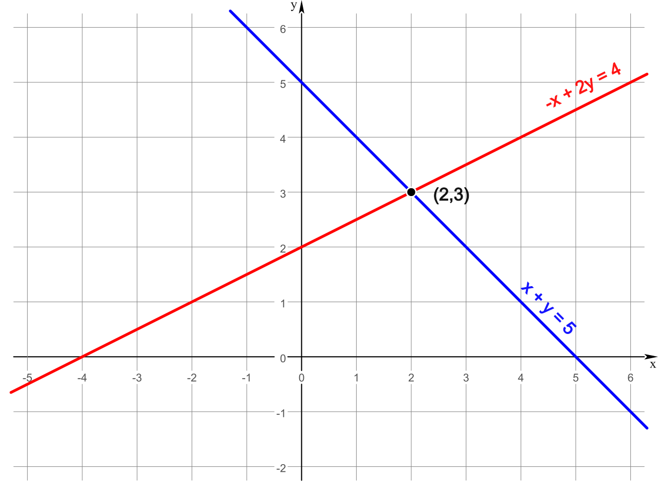
When the two sides of a linear equation are graphed as independent lines, a single solution corresponds geometrically to their exact point of intersection on the coordinate plane.

2. No Solution Sometimes, the algebra yields an absurdity. A one-variable linear equation has no solution if algebraic simplification results in a mathematically false statement such as $0 = 1$ . When this happens, it means no real number exists that can satisfy the initial conditions. The equation represents a logical impossibility.

3. Infinitely Many Solutions Conversely, the variable might vanish entirely, leaving a tautology. A one-variable linear equation has infinitely many solutions if algebraic simplification results in a mathematically true statement such as $0 = 0$ . This indicates the original equation was an identity—a mathematical equation that remains true for all possible values of the substituted variables.

If an equation is a balanced scale, an inequality is a scale tipped permanently in one direction. Solving linear inequalities utilizes almost identical logic to equations, with one vital distinction.

The rules that mirror equations perfectly:

The Addition Property of Inequality: Adding the same number to both sides of an inequality preserves the original direction of the inequality symbol.
The Subtraction Property of Inequality: Subtracting the same number from both sides of an inequality preserves the original direction of the inequality symbol.
Multiplying both sides of a linear inequality by a positive number preserves the direction of the inequality symbol.
Dividing both sides of a linear inequality by a positive number preserves the direction of the inequality symbol.

The Addition Property of Inequality visualized on a number line: shifting both values by the same constant preserves their relative order and spatial relationship.

The Great Reversal

Here is the concept that universally trips up middle school students: multiplying or dividing by a negative number.

Multiplying both sides of a linear inequality by a negative number reverses the direction of the inequality symbol.
Dividing both sides of a linear inequality by a negative number reverses the direction of the inequality symbol.

Why? Do not let your students memorize this blindly. Use the number line. The numbers $3$ and $5$ exist on the right side of zero, and $3 < 5$ . When we multiply by $-1$ , we reflect these values across zero. They become $-3$ and $-5$ . Because $-5$ is further to the left, it is lesser. The relationship has flipped: $-3 > -5$ . Negative multiplication is a mirror reflection of the number line, and mirrors reverse images.

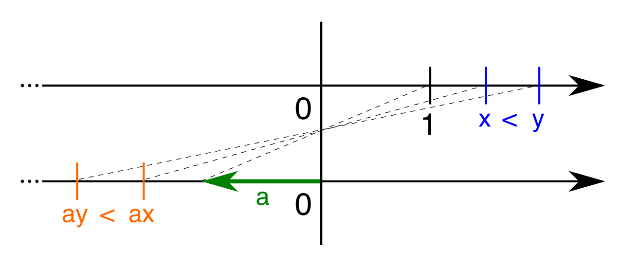
Multiplying an inequality by a negative number reflects the values across zero on the number line, requiring the inequality symbol to reverse direction to maintain mathematical truth.

Because inequalities often possess infinitely many solutions (e.g., $x > 3$ ), we cannot simply write a single number. We must map the solution set visually.

On a one-dimensional number line, the boundary of the solution is marked by a circle:

A strictly greater than symbol ( $>$ ) is graphically represented by an open, unshaded circle. This indicates the boundary value itself is not included.
A strictly less than symbol ( $<$ ) is similarly graphically represented by an open, unshaded circle.
A greater than or equal to symbol ( $\ge$ ) is graphically represented by a closed, solid circle, meaning the boundary value is included in the solution.
A less than or equal to symbol ( $\le$ ) is graphically represented by a closed, solid circle.

Once the boundary is established, we shade the line to capture the infinite possibilities:

The solution set to an inequality of the form $x > a$ is graphed by shading all points to the right of the value $a$ on a number line.
The solution set to an inequality of the form $x < a$ is graphed by shading all points to the left of the value $a$ on a number line.

Eventually, middle school curricula push into two dimensions. When a one-variable inequality is ported into the Cartesian coordinate system (the xy-plane), the visual representation expands. A single-variable linear inequality graphed in the two-dimensional xy-plane visually forms a shaded region known as a half-plane.

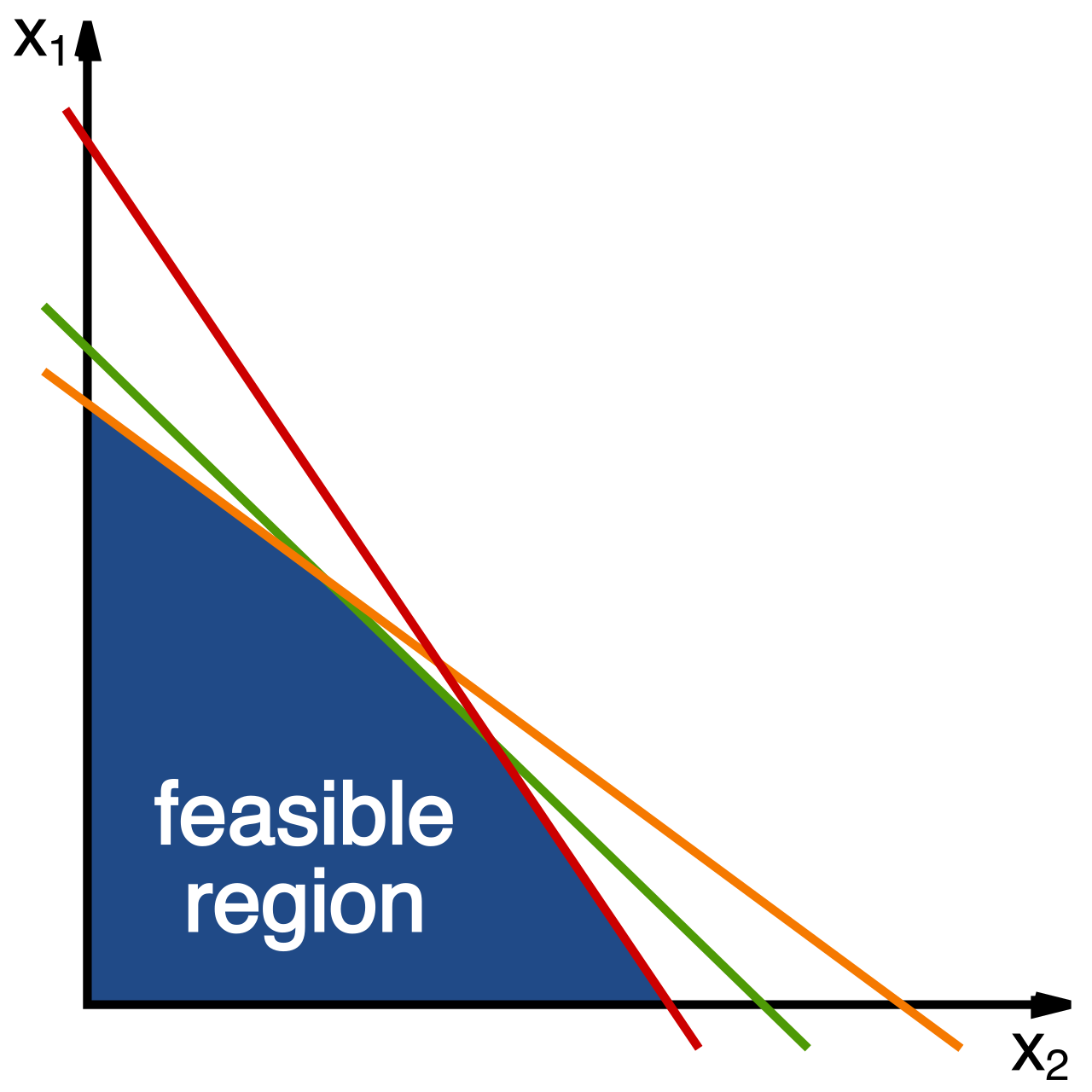
In a two-dimensional Cartesian coordinate system, linear inequalities are represented as shaded half-planes. The overlapping areas define the viable solution set for a system of inequalities.

Just as open and closed circles delineate strict vs. inclusive boundaries on a 1D line, we use different types of lines in 2D space:

In the xy-plane, an inequality utilizing a strictly greater than or strictly less than symbol is visually bounded by a dashed line. The dash tells the observer, "Approach this boundary, but do not touch it."
In the xy-plane, an inequality utilizing a greater than or equal to symbol or a less than or equal to symbol is visually bounded by a solid line.

Consider how one-variable inequalities behave in this 2D space:

Inequality Format	Boundary Line Style	Graphical Representation in the xy-Plane
$x > a$	Dashed, Vertical	The one-variable inequality $x > a$ graphed in the xy-plane is depicted as a dashed vertical line with the entire half-plane to the right of the line shaded. Every $(x, y)$ coordinate in this infinite rightward expanse has an $x$ -value larger than $a$ .
$y < b$	Dashed, Horizontal	The one-variable inequality $y < b$ graphed in the xy-plane is depicted as a dashed horizontal line with the entire half-plane below the line shaded. Here, every point shares the property that its height ( $y$ ) is less than the boundary $b$ .

Understanding these structures conceptually—rather than as rote steps—allows you to debug your students' misconceptions in real-time. Whether translating a physical scale into properties of equality or projecting a one-dimensional inequality into an infinite two-dimensional half-plane, you are illuminating the strict, beautiful logic that holds mathematics together.