Algebraic Expressions and Polynomials

Not sure you’re ready?

Take the ~3-minute readiness diagnostic and see where you stand.

When a master mechanic opens the hood of a car, they do not see a single, indivisible block of metal; they see a system of interlocking components—belts, gears, and cylinders—that can be dismantled, inspected, and reassembled to alter the machine's performance. An algebraic expression is precisely the same kind of machinery: a mathematical phrase containing numbers, variables, and operational symbols without an equal sign. By manipulating its structure, we reveal its behavior. When we ask our secondary students to simplify or rewrite these phrases, we are teaching them how to rebuild the engine to run more efficiently. If they want to test if their newly rebuilt engine matches the original, they must verify that they have created equivalent algebraic expressions, which yield identical numerical values for every possible valid substitution of variables in the domain. The ultimate test of this machinery is evaluating a specific algebraic expression, which requires substituting concrete numerical values for the present variables and subsequently computing the arithmetic result.

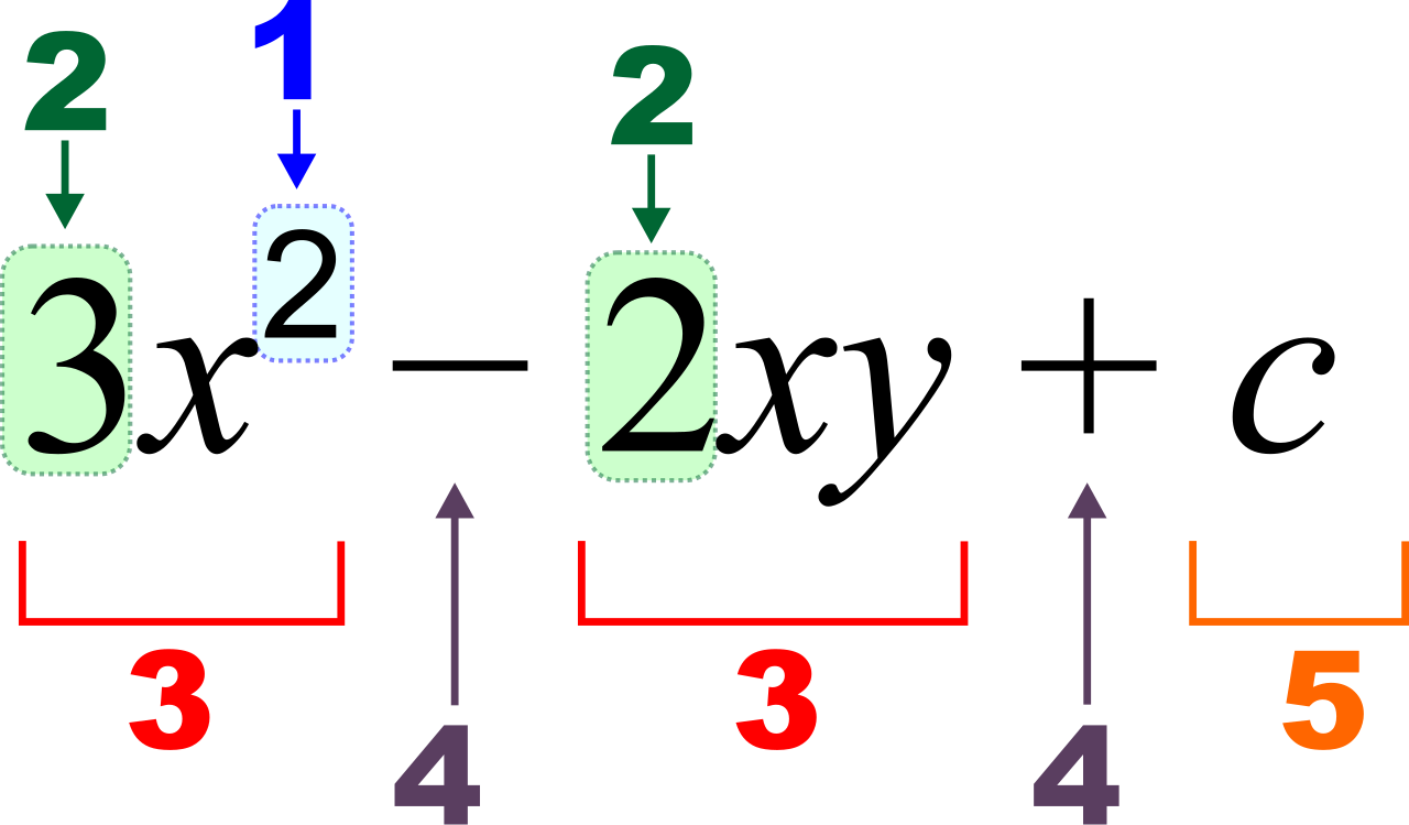
Just as a mechanic identifies the parts of an engine, students must identify the structural components of an algebraic expression, such as coefficients, variables, and exponents.

To truly understand algebraic structures, we must first establish the boundaries of the environment in which we are operating. The most ubiquitous structures in secondary mathematics are polynomials. A polynomial is a mathematical expression consisting of variables and coefficients connected using exclusively addition, subtraction, and non-negative integer exponents.

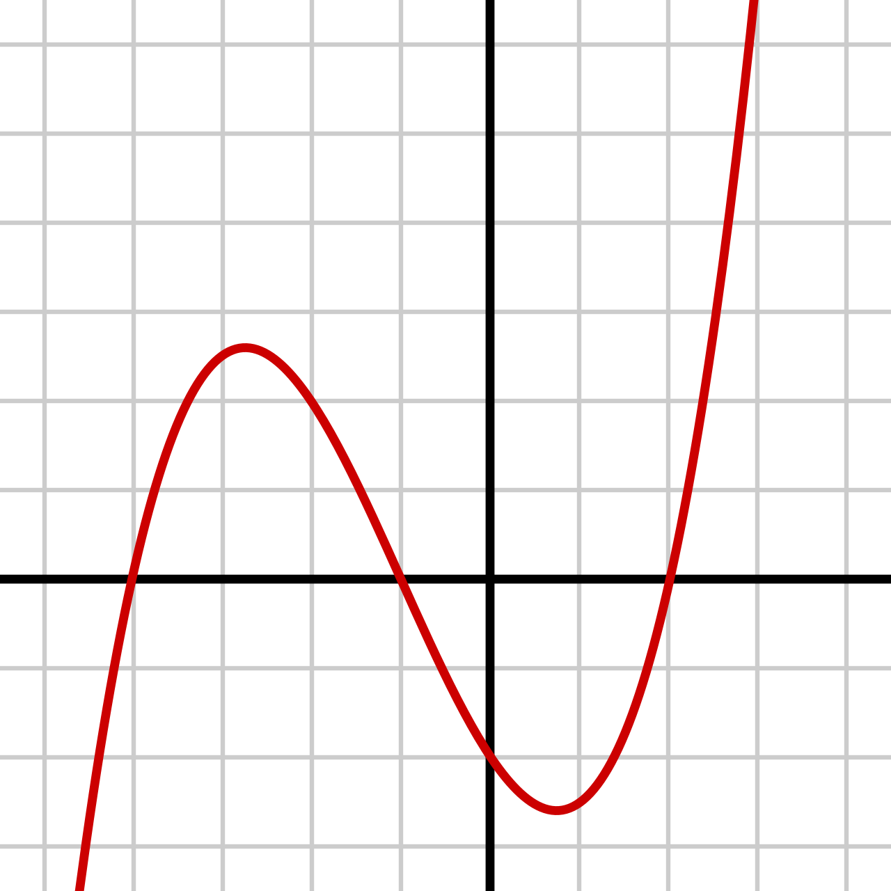
Because we only allow non-negative integer exponents, polynomials behave beautifully. They are smooth, continuous, and predictable. The behavior of a single-variable polynomial at its extremes—what your students will see when they zoom out on a graphing calculator—is governed by its degree, which is determined by the highest exponent of the variable present in the entire expression.

The macroscopic behavior of a polynomial, such as this degree-three curve, is entirely dictated by the highest exponent of its variable.

The Power of Closure

In mathematics, an environment is "closed" under an operation if performing that operation on elements within the set always produces another element that belongs to the same set. Think of it like a biological ecosystem: if two organisms breed and produce an organism of the exact same species, the system is closed.

Because polynomials are essentially built from repeated addition and multiplication, they possess robust structural integrity:

The mathematical set of polynomials exhibits strict closure under the operation of addition.
The mathematical set of polynomials exhibits strict closure under the operation of subtraction.
The mathematical set of polynomials exhibits strict closure under the operation of multiplication.

However, the ecosystem breaks open when we introduce division. The mathematical set of polynomials does not exhibit closure under the operation of division.

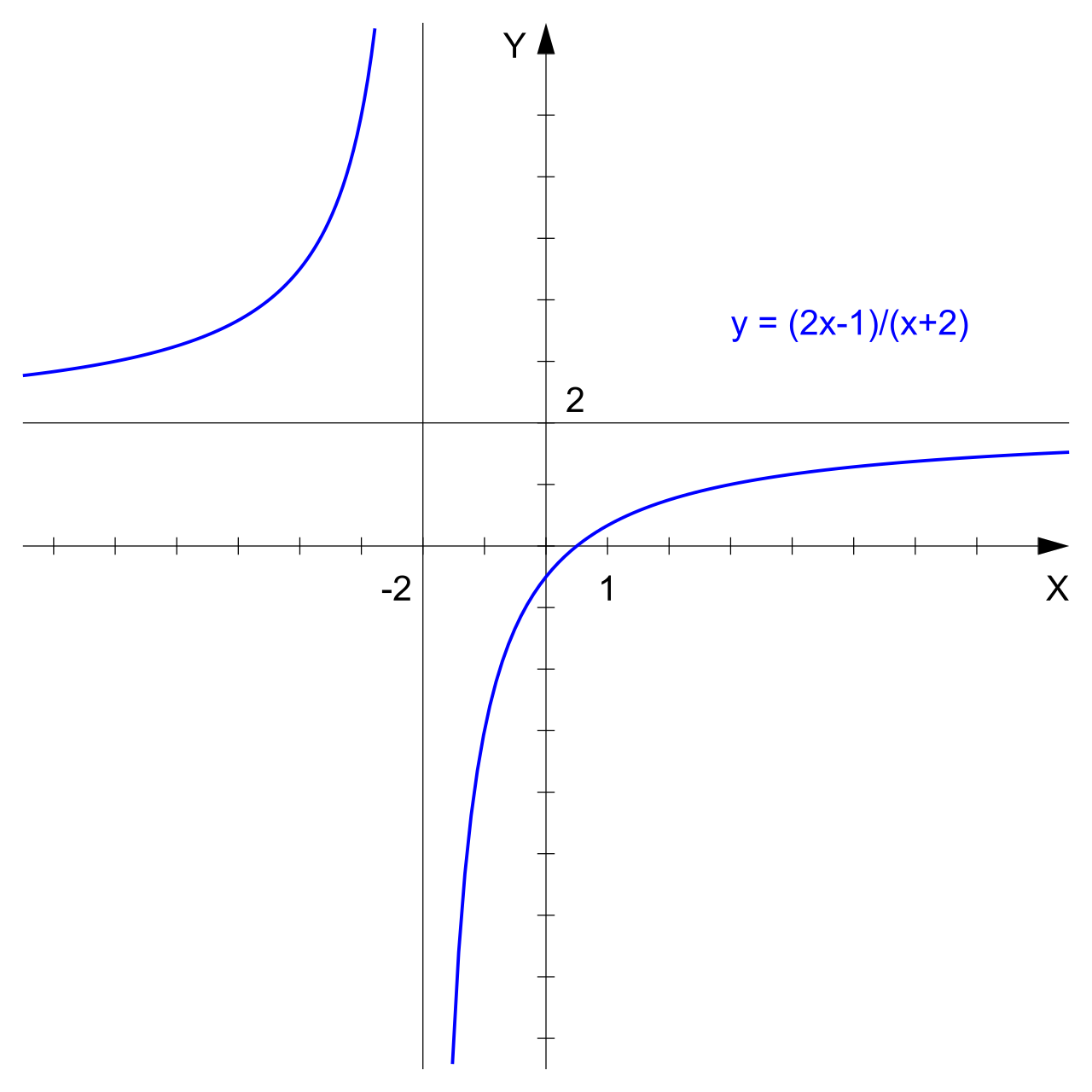
Dividing one polynomial by another polynomial can produce a rational algebraic expression instead of a polynomial. A rational algebraic expression is formally defined in mathematics as the algebraic ratio of two individual polynomials. This creates a pedagogical bridge: just as dividing integers necessitates the creation of fractions, dividing polynomials necessitates the creation of rational expressions.

When your students graph these rational functions, they will inevitably encounter asymptotes and "domain errors." This occurs because the valid domain of a rational algebraic expression strictly excludes any input values causing the denominator polynomial to evaluate to zero. Recognizing and finding these domain boundaries is a critical skill for secondary students, as it connects algebraic manipulation directly to graphical behavior.

Dividing polynomials often yields rational functions. The domain of these functions excludes x-values that make the denominator zero, creating vertical asymptotes where the graph breaks.

When we perform arithmetic on polynomials, we are relying on foundational axioms of real numbers.

Adding polynomials requires computing the combined sum of numerical coefficients for terms possessing identical variable parts. This process, universally known as combining like terms, simplifies expressions by adding the numerical coefficients of terms with identical variable components. It is nothing more than the distributive property in reverse: $3x^2 + 5x^2 = (3+5)x^2 = 8x^2$ .

Subtracting polynomials requires distributing a negative one to every individual term in the subtrahend polynomial before combining like terms. This is where novice algebra students routinely stumble. They will subtract the leading term but forget the rest of the polynomial. Framing subtraction as "adding the distributed negative" resolves this structural error.

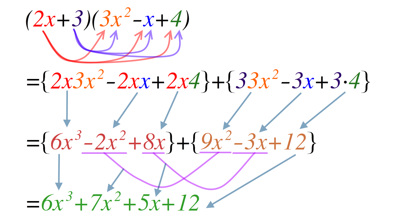
To push outward, we multiply. Multiplying two polynomials requires distributing every individual term in the first polynomial to every individual term in the second polynomial. This relies fundamentally on the distributive property, which allows multiplying a sum by a single term by multiplying each individual addend by that single term.

When we apply this exhaustively, we are expanding an algebraic expression, which removes parentheses by completely applying the distributive property across all present terms.

Expanding a polynomial requires exhaustive application of the distributive property, multiplying each term in the first polynomial by every term in the second.

If expanding is driving the car, factoring is taking the engine apart to see how it works. Factoring an algebraic expression rewrites an expanded sum or difference as a mathematical product of simpler factors.

Before deploying complex algorithms, a disciplined mathematician always looks for the simplest component first. The greatest common factor of a polynomial is the largest single monomial expression that divides evenly into all individual terms of the polynomial. Consequently, extracting the greatest common algebraic factor is the standard preliminary step in completely factoring any given polynomial expression.

Factoring Quadratics and Grouping

When confronting a trinomial, your students must recognize the hidden combinations of coefficients. A quadratic expression taking the mathematical form $ax^2 + bx + c$ can be factored by identifying two numerical values multiplying to $ac$ and summing to $b$ .

For polynomials with four terms, we deploy a strategic division of labor. Factoring by grouping is an algorithmic technique involving grouping terms with common factors before factoring out a shared binomial factor. It is essentially the distributive property applied to blocks of terms rather than individual monomials.

Special Polynomial Forms

Certain polynomials possess symmetries that allow us to bypass standard algorithms. Recognizing these forms is crucial for speed and accuracy on standardized assessments.

Name	Factored Form	Conceptual Note
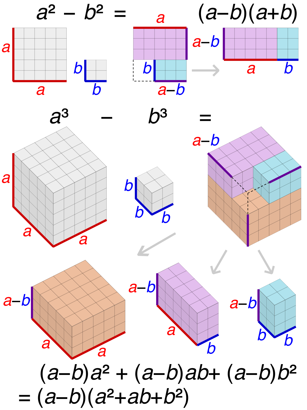
Difference of Two Squares	$a^2 - b^2 = (a - b)(a + b)$	The middle terms cancel out perfectly due to opposing signs.
Perfect Square Trinomial (Positive)	$a^2 + 2ab + b^2 = (a + b)^2$	A perfect square trinomial with a positive middle term factors according to this algebraic formula.
Perfect Square Trinomial (Negative)	$a^2 - 2ab + b^2 = (a - b)^2$	A perfect square trinomial with a negative middle term factors according to this algebraic formula.
Difference of Two Cubes	$a^3 - b^3 = (a - b)(a^2 + ab + b^2)$	The difference of two cubes formula states that $a^3 - b^3$ factors into the product $(a - b)(a^2 + ab + b^2)$ .
Sum of Two Cubes	$a^3 + b^3 = (a + b)(a^2 - ab + b^2)$	The sum of two cubes formula states that $a^3 + b^3$ factors into the product $(a + b)(a^2 - ab + b^2)$ .

Geometric visualizations can provide intuitive proofs for special polynomial factorization patterns, such as the difference of two squares and the difference of two cubes.

Eventually, we encounter polynomials that refuse to yield. Irreducible polynomials fundamentally cannot be factored into non-constant polynomials of lower degree over a specified mathematical number field.

Consider the expression $a^2 + b^2$ . The sum of two squares algebraic expression $a^2 + b^2$ cannot be factored into real binomial factors using purely real numbers. If we restrict our students to the real number line, $x^2 + 4$ is irreducible.

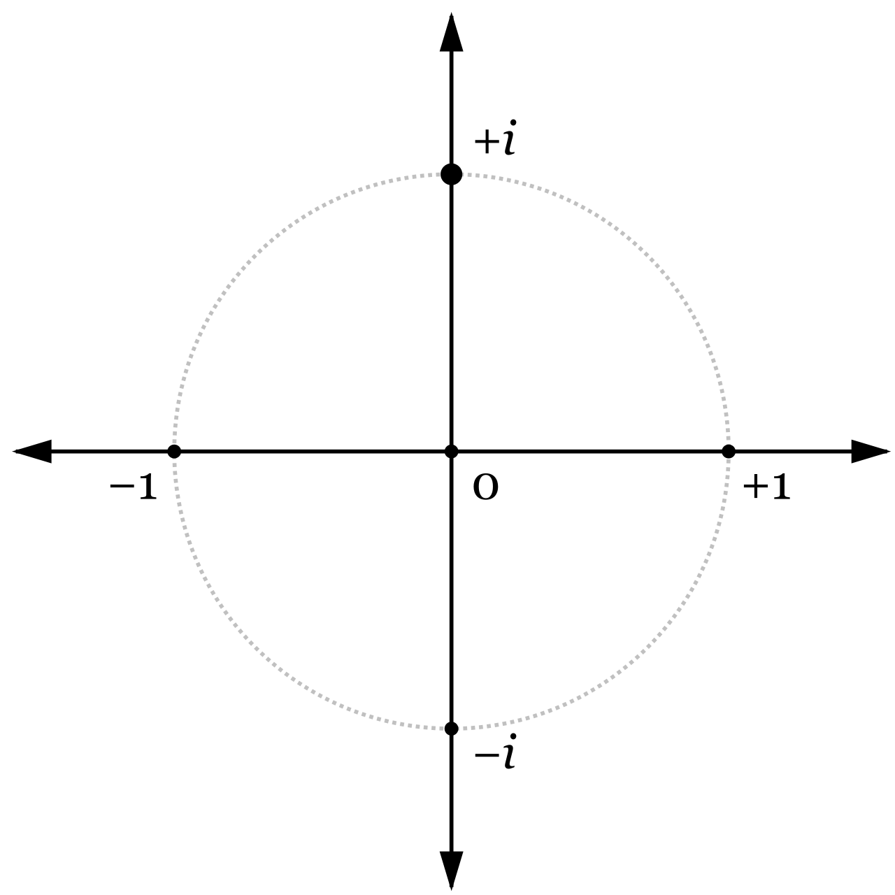
However, mathematics rarely accepts a locked door without inventing a key. To factor a sum of squares, we must expand our number system. The imaginary unit $i$ is mathematically defined as the principal square root of negative one. Consequently, the mathematical square of the imaginary unit $i$ is exactly equal to negative one ( $i^2 = -1$ ).

By introducing complex numbers, the locked door opens: the sum of two squares formula over complex numbers states that $a^2 + b^2$ factors into the product $(a - bi)(a + bi)$ . When we multiply this out, the inner and outer terms cancel, and the final term becomes $-b^2 i^2$ , which simplifies beautifully back to $+b^2$ .

Expanding our number system to include the imaginary unit i allows us to factor sums of squares by visualizing roots on the complex plane.

Division is the tool we use to break polynomials down, and it comes in two distinct mechanical varieties.

Polynomial long division is a systematic algorithm used to divide a dividend polynomial by a divisor polynomial of equal or lower degree. It perfectly mimics base-10 integer long division, emphasizing place value (degree) at every step.

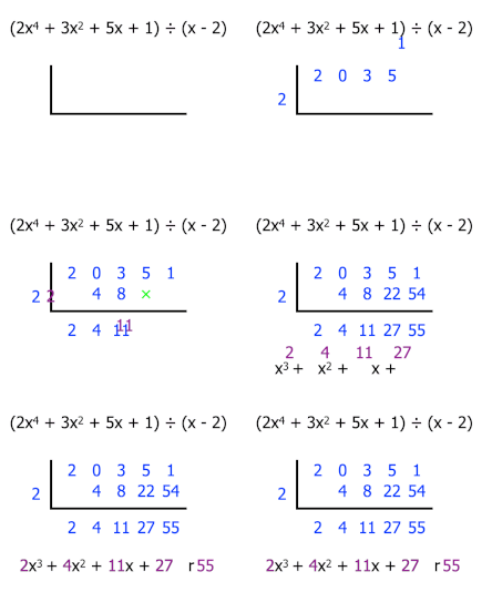
When the divisor is particularly simple, we can strip away the variables and operate solely on the coefficients. Synthetic division is a condensed computational method strictly utilized for dividing a polynomial by a linear monic binomial (an expression of the form $x - c$ ).

Synthetic division offers a highly efficient, algorithmic shortcut for dividing a polynomial by a linear binomial, tracking only the structural coefficients.

Regardless of the method used, the result always obeys a fundamental structural law:

The polynomial division algorithm states that a dividend polynomial equals the product of the divisor and quotient polynomials added to a remainder polynomial. $P(x) = D(x)Q(x) + R(x)$

To maintain logical consistency, in the polynomial division algorithm, the mathematical degree of the remainder polynomial must be strictly less than the degree of the divisor polynomial. If it weren't, we could divide one more time.

The Remainder and Factor Theorems

The division algorithm gives birth to two of the most elegant and interconnected theorems in algebra.

Imagine we divide a polynomial $P(x)$ by a linear binomial $(x - c)$ . The degree of the divisor is 1, meaning the remainder must have a degree of 0—it must be a constant, $r$ . Thus, $P(x) = (x - c)Q(x) + r$ . What happens if we evaluate the polynomial at $x = c$ ? The $(c - c)$ term becomes zero, annihilating the quotient $Q(c)$ , and leaving only $r$ .

This is the brilliant simplicity of The Remainder Theorem: it states that dividing a polynomial by a linear binomial $x - c$ yields a constant remainder equal to the polynomial evaluated at $c$ . ( $P(c) = r$ ).

This directly implies its natural successor. If the remainder is zero, the division was perfect, meaning $(x - c)$ is a clean factor. Therefore, the Factor Theorem states that a linear binomial $x - c$ perfectly divides a polynomial if and only if evaluating the polynomial at $c$ yields zero.

These theorems are essential for secondary teachers. They provide a vital computational shortcut: instead of executing a lengthy division algorithm to check if $(x - 5)$ is a factor of a massive polynomial, a student can simply evaluate $P(5)$ using their calculator. If the result is zero, it's a factor.

Finding factors is inextricably linked to finding roots (x-intercepts, or zeros). The theoretical ceiling of this pursuit is established by the crown jewel of polynomial mathematics.

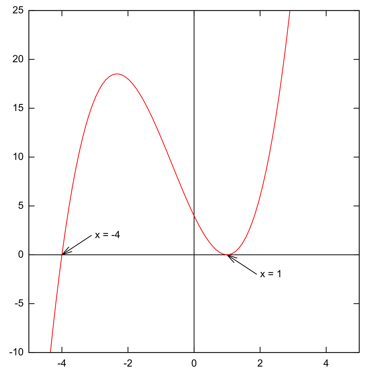
The Fundamental Theorem of Algebra states that every non-zero single-variable polynomial of degree $n$ has exactly $n$ complex roots. This theorem is a guarantee. A 5th-degree polynomial has exactly 5 complex roots, accounting for multiplicity. Some of those roots may be real, crossing the x-axis on a graphing calculator, while others may be purely complex, existing beyond the real plane.

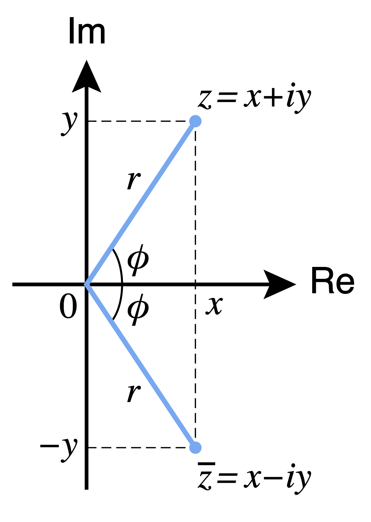
The multiplicity of a polynomial's roots dictates its graphical interaction with the x-axis: single roots cross straight through, while even-multiplicity roots merely touch and turn around.

When complex roots do appear in polynomials that feature standard, real-world parameters, they behave with strict, mirrored discipline. Complex conjugate roots always occur in pairs for any mathematical polynomial possessing exclusively real coefficients. This means that for any real-coefficient polynomial possessing a complex root $a + bi$ , the complex conjugate $a - bi$ is guaranteed to be a root of the identical polynomial. It is structurally impossible for a real-coefficient polynomial to have $3+2i$ as a root without also possessing $3-2i$ as a root; they must cancel out each other's imaginary components during expansion to preserve the real coefficients.

In polynomials with strictly real coefficients, any complex roots are structurally obligated to appear in conjugate pairs, mirroring each other across the real axis.

The Rational Root Theorem

Before graphing calculators made finding real roots trivial, mathematicians required a method to narrow down the infinite possibilities of real numbers into a finite, testable list. We still teach this today to build a student's number sense regarding polynomial structure.

The Rational Root Theorem provides a finite list containing all theoretically possible rational roots of a polynomial equation featuring integer coefficients.

How is this list built? Look at the factored form of a polynomial. The constant term of the expanded polynomial is always the product of the constant terms of the factors, and the leading coefficient is always the product of the leading coefficients of the factors. Therefore: Possible rational roots of an integer-coefficient polynomial are generated by dividing a factor of the constant term by a factor of the leading coefficient. ( $\frac{p}{q}$ ).

For an aspiring mathematics educator, mastering these structures is not just about passing an exam; it is about grasping the underlying machinery of algebraic thought. When you can fluently translate between an expanded polynomial, its factored form, its roots, and its graphical representation, you empower your students to stop memorizing disconnected rules and start seeing the beautifully interconnected architecture of mathematics.