Creating Equations and Inequalities

Not sure you’re ready?

Take the ~3-minute readiness diagnostic and see where you stand.

When a civil engineer designs the load-bearing cables of a suspension bridge, or an epidemiologist forecasts the spread of a pathogen, they do not rely on trial and error. They build their realities first in the profound, invisible language of mathematics. They take the messy, chaotic physical world—steel tension, human interactions, time, space—and distill it into clean syntax. As an aspiring mathematics educator, your ultimate task is not merely to teach students how to manipulate symbols on a page; it is to teach them how to translate the universe into those symbols, and then how to translate the algebraic results back into the physical world.

John Snow's 1854 map of cholera clusters illustrates how early epidemiologists translated the chaotic physical spread of a pathogen into a clear mathematical model.

To master the creation of equations and inequalities for the Praxis 5165 exam, we must look at algebra not as a collection of arbitrary rules, but as a precise descriptive physics. We are mapping relationships, defining boundaries, and establishing constraints.

Before we can solve a problem, we must articulate it. The process of modeling a real-world situation requires defining all variables explicitly along with the corresponding units of measure. If a student writes $x = 5$ , it means nothing. If they write Let $x$ represent the time elapsed in seconds, they have successfully tethered the abstract symbol to physical reality. Translating a scenario into an equation involves identifying the unknown quantity and assigning a specific variable to that quantity.

At its core, an algebraic equation is a mathematical statement asserting the equality of two expressions. When you write an equals sign, you are making a profound claim. You are declaring that two seemingly different expressions are merely masks for the exact same underlying value. In the translation from English to algebra, the word "is" in a word problem typically translates to the equals sign in an algebraic equation.

The first recorded use of an equals sign, published in 1557, established the mathematical syntax for declaring that two seemingly different expressions share the exact same underlying value.

Families of One-Variable Equations

Different physical phenomena require different mathematical architecture. We capture these via specific function families in one variable:

Linear Equations: Creating a one-variable linear equation requires identifying a constant rate of change and an initial value from a given scenario. If a plumber charges a $50 diagnostic fee plus $75 per hour, the initial value is 50, and the constant rate is 75.
Quadratic Equations: Nature rarely moves in straight lines. Quadratic equations in one variable are used to model real-world scenarios involving area, optimization, or projectile motion. When you want to know exactly when a basketball will hit the gymnasium floor, you set a one-variable quadratic expression (representing height) equal to zero.
Exponential Equations: Growth is often compounded. Exponential equations in one variable model scenarios involving a constant percentage rate of growth or a constant percentage rate of decay. Think of a savings account growing by 4% annually or carbon-14 decaying in an archeological artifact.
Rational Equations: Rational equations in one variable are used to model shared work-rate problems or average cost calculations. If it takes Teacher A three hours to grade exams alone, and Teacher B four hours, a rational equation $\frac{1}{3} + \frac{1}{4} = \frac{1}{t}$ captures the reality of their combined labor.

Defining Boundaries: Inequalities in One Variable

Sometimes, we are not looking for a single perfect match; we are establishing a boundary.

Inequalities are the mathematical language of limits. When reading a scenario, the phrase "at least" in a word problem translates to the greater than or equal to mathematical inequality symbol ( $\geq$ ), while the phrase "at most" in a word problem translates to the less than or equal to mathematical inequality symbol ( $\leq$ ).

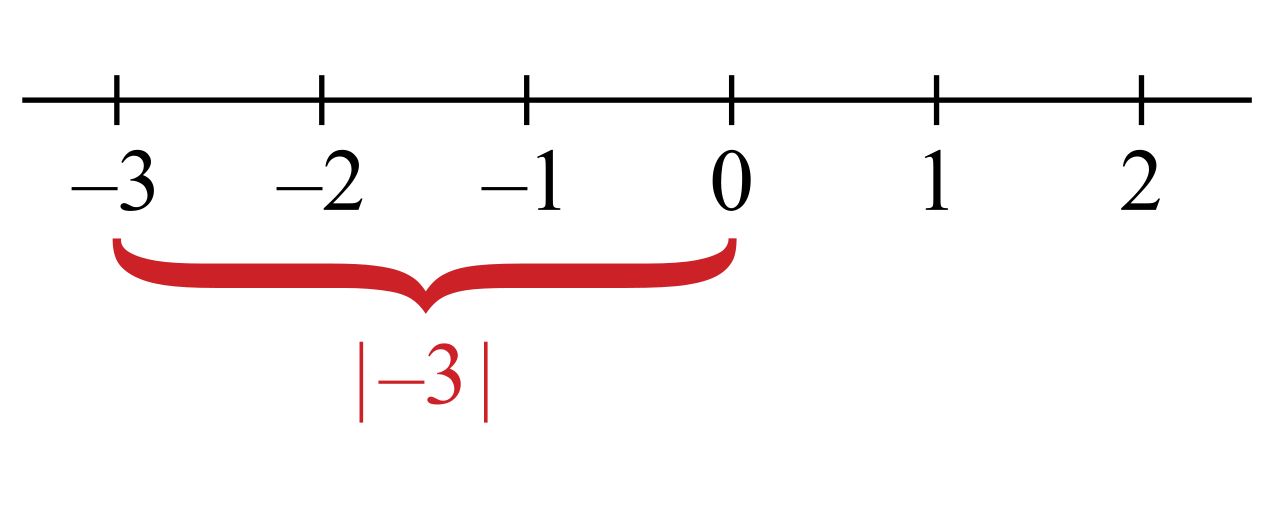
A particularly elegant form of boundary setting involves absolute value. Absolute value inequalities in one variable model scenarios involving a specified margin of error or tolerance from a target value. If a factory machines a piston ring that must be 80 millimeters wide, with an allowable tolerance of 0.05 millimeters, the inequality $|x - 80| \leq 0.05$ perfectly captures this margin of error. It mathematically states, "The distance between our actual size and our target size must be no more than our tolerance."

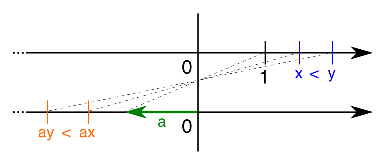
Because absolute value represents physical distance from a target center, it is the ideal mathematical tool for defining margins of error and establishing manufacturing tolerances.

The Reversal Axiom: When solving these boundaries, multiplying or dividing an algebraic inequality by a negative number requires reversing the direction of the inequality symbol. Why does this matter? Think of a number line. Multiplying by a negative number reflects our position across zero. If 5 is to the right of 3 ( $5 > 3$ ), reflecting them across zero places $-5$ to the left of $-3$ ( $-5 < -3$ ). The structural relationship flips, so our syntax must flip to remain truthful to reality.

Multiplying or dividing by a negative number reflects the position of values across zero on a number line, structurally flipping their relationship and requiring a reversal of the inequality symbol.

The world is rarely static. Usually, one condition depends entirely on another. An equation in two variables defines a relationship where the value of a dependent variable changes based on the value of an independent variable.

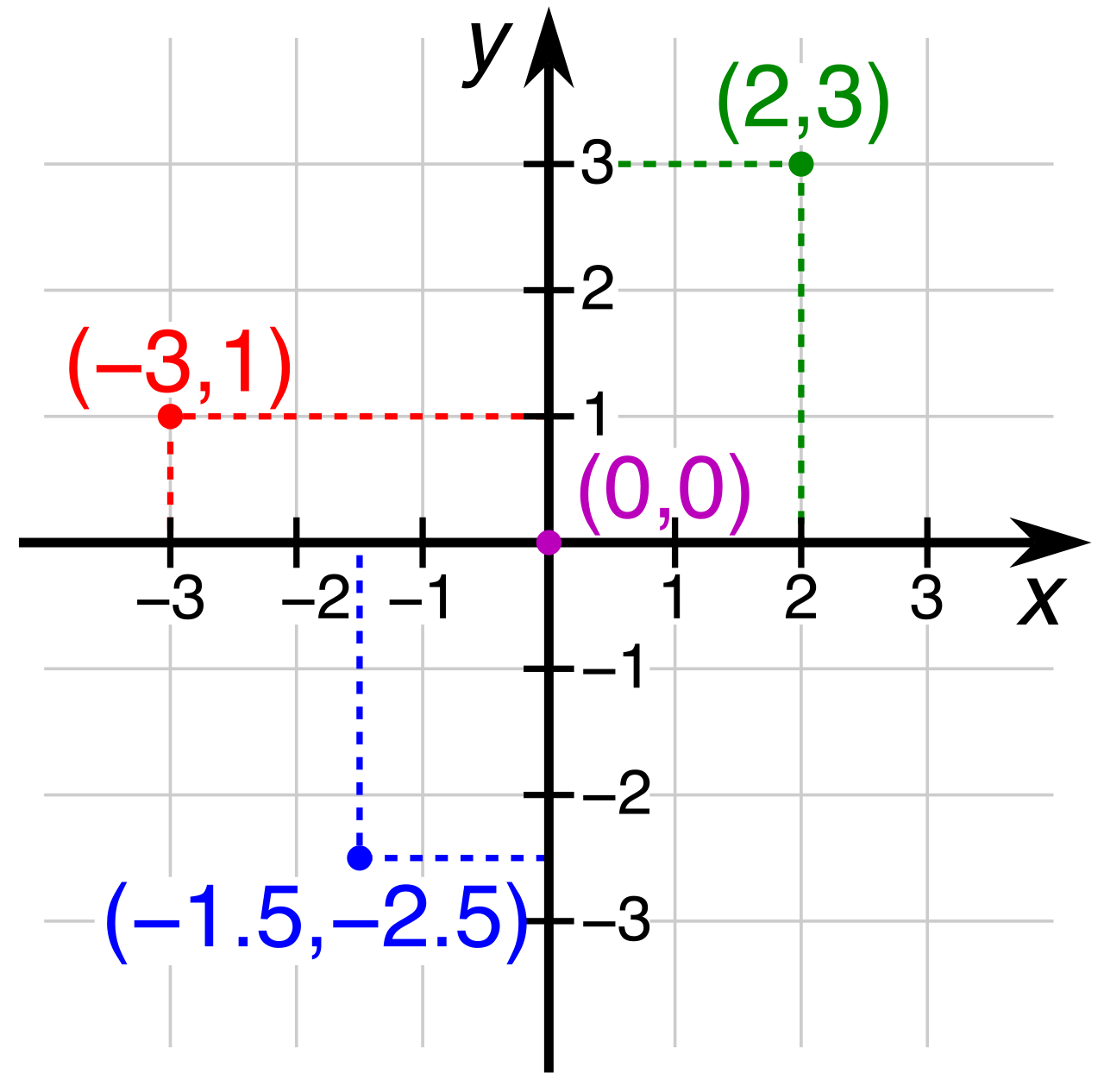
Because human beings are visual creatures, we need a way to see this relationship. The coordinate plane is used to visually represent equations and inequalities containing exactly two variables. It translates algebra into geometry.

The Cartesian coordinate plane provides the geometric architecture necessary to visually map out dynamic relationships between independent and dependent variables.

The Architectures of Two-Variable Relationships

When mapping dynamic relationships, we look for how the variables interact mathematically:

Linear Relationships: A linear equation in two variables is used when the rate of change between the independent and dependent variables is constant. You must be fluent in translating between the three primary forms depending on the information provided in the scenario:
- Standard Form: The standard form of a linear equation in two variables is $Ax + By = C$ . This is ideal for scenarios involving combinations of two distinct items, like buying $x$ adult tickets and $y$ student tickets for a total cost of $C$ .
- Slope-Intercept Form: The slope-intercept form of a linear equation in two variables is $y = mx + b$ . This is the workhorse of graphing, explicitly isolating the dependent variable.
- Point-Slope Form: The point-slope form of a linear equation in two variables is $y - y_1 = m(x - x_1)$ . This is often the most efficient bridge between raw data (a single occurrence and a rate) and an algebraic model.
Proportional Variations: Often, we deal with direct relationships. Direct variation models require a two-variable equation where the dependent variable is a constant multiple of the independent variable ( $y = kx$ ). Conversely, inverse variation models require a two-variable equation where the product of the independent and dependent variables is a constant ( $xy = k$ , or $y = \frac{k}{x}$ ). If a school hires more contractors, the time required to build the new library decreases—an inverse variation.
Exponential Relationships: When a virus spreads or a rumor cascades through a high school, the rate of change is not constant. An exponential equation in two variables is used when the dependent variable changes by a constant multiplicative factor for each unit change in the independent variable.
Quadratic Relationships: If you give your students a table of raw data, how do they know it forms a parabola? A quadratic equation in two variables models mathematical relationships exhibiting a constant second difference. If the rate of the rate of change is constant, gravity or area is likely at play.

Mapping Regions: Two-Variable Inequalities

When dealing with two variables, an inequality doesn't just give us a line; it gives us an entire territory. An inequality in two variables represents a boundary line and a shaded region containing all ordered pairs that satisfy the inequality.

The border of this territory must be carefully defined. The boundary line of a two-variable inequality is drawn as a solid line for inclusive inequalities ( $\geq$ or $\leq$ ), indicating that the border itself is part of the solution territory. Conversely, the boundary line of a two-variable inequality is drawn as a dashed line for strict inequalities ( $>$ or $<$ ), acting merely as a fence that the solutions may approach but never touch.

In the real world, we rarely operate under a single condition. A business has a limit on both its budget and its labor hours. Mathematical constraints are conditions or restrictions placed on the variables within a mathematical model.

To handle overlapping realities, we use systems. A system of equations consists of two or more equations that share the same set of variables. When you solve a system, you are hunting for the exact moment where multiple independent realities agree.

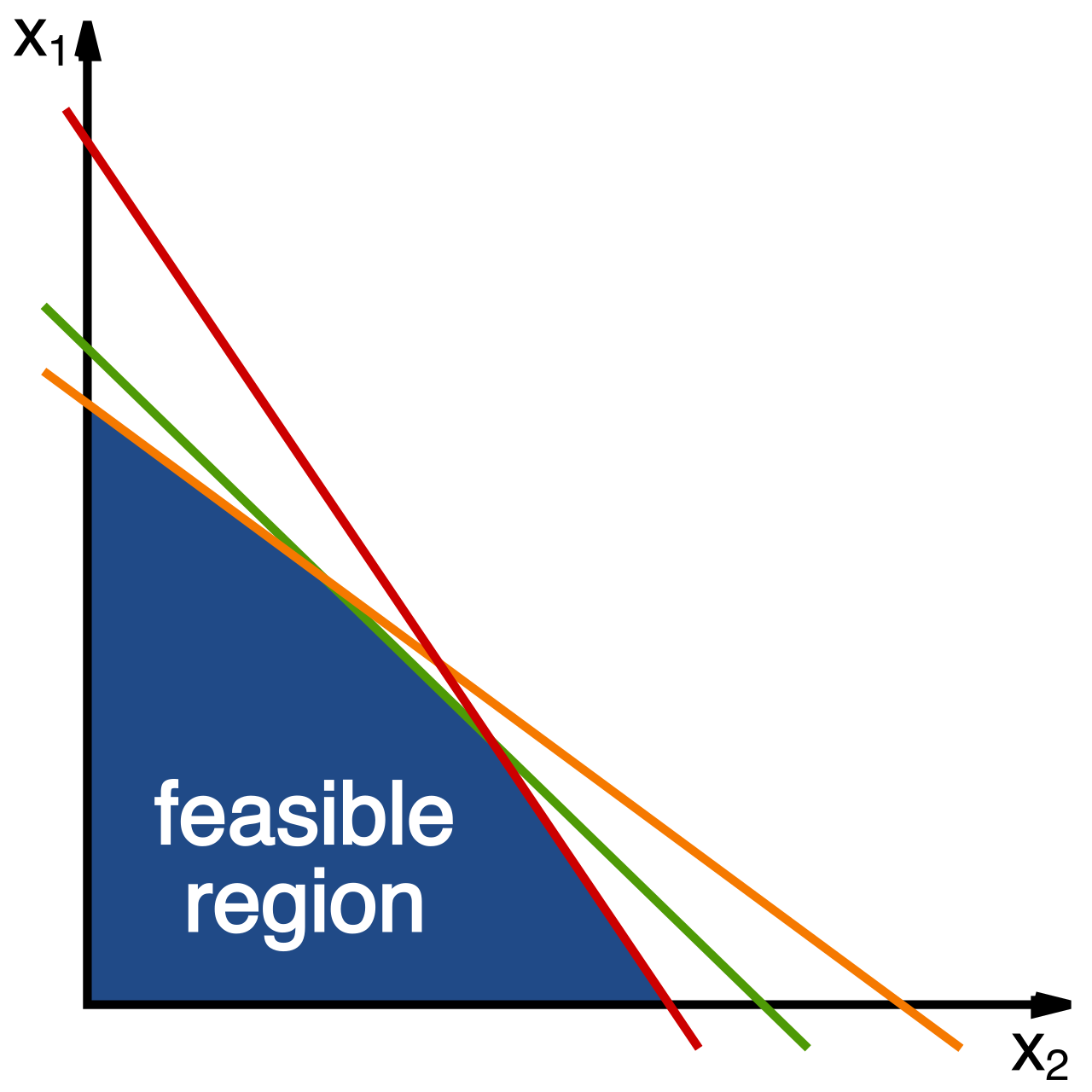
Furthermore, constraints in a real-world scenario can be represented algebraically by a system of linear equations or a system of linear inequalities. When we graph a system of inequalities, the overlapping shaded areas create something highly specific. The solution set to a system of linear inequalities forms a feasible region on the coordinate plane.

Why do we care about this region? In operations research, logistics, and daily decision-making, a feasible region contains all possible combinations of variable values that satisfy all given mathematical constraints simultaneously. Any point inside this region is a scenario that physically "works" without breaking your budget, time limit, or material constraints.

The overlapping shaded areas of a system of linear inequalities define a bounded feasible region, containing all sets of variables that physically work within given constraints.

Here is the most critical lesson for any student using a graphing calculator: algebra is blind to reality. The algebra will eagerly give you an answer to the equation you typed. But the algebra does not know you are calculating the flight of a rocket, the number of buses required for a field trip, or the mass of a chemical compound.

Therefore, an algebraic solution to a mathematical model must be evaluated to determine whether the solution is a viable option in the real-world context.

A number might balance the equation perfectly, but fail the test of physical reality. A viable solution must fall within the practical domain of the real-world scenario being modeled. The mathematical domain might be all real numbers ( $\mathbb{R}$ ), but the practical domain is restricted by the universe we live in.

Recognizing Non-Viable Solutions

You and your students must actively interrogate the solutions you generate. Watch for these common pitfalls:

Type of Non-Viable Solution	The Reality Check	Example
Negative Solutions	Negative algebraic solutions are non-viable in real-world models involving exclusively positive quantities like elapsed time, geometric distance, or physical mass.	A quadratic formula tells you a ball hits the ground at $t = 3$ seconds and $t = -1.5$ seconds. The $-1.5$ is mathematically true to the parabola, but physically impossible, as time cannot be negative.
Fractional Solutions	Fractional algebraic solutions are non-viable in models that require discrete whole quantities such as the number of living people or manufactured items.	If your system of equations reveals you need $4.2$ buses to transport the debate team, $4.2$ is non-viable. You must rent $5$ buses.

The Illusion of Extraneous Solutions

Sometimes the algebra isn't just physically impossible; it is a mathematical ghost created by our own solving methods. Extraneous solutions are mathematically correct roots of an algebraic process that do not satisfy the original contextual constraints of the model.

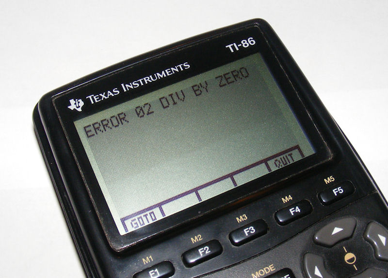
When we square both sides of a radical equation, or multiply by a variable denominator in a rational equation, we sometimes unintentionally create a new, broader equation that includes answers the original equation explicitly forbids (such as causing division by zero). These are extraneous.

Calculators will blindly evaluate algebraic syntax, halting only for undefined physical limits like division by zero—which often signals an extraneous solution in a generated model.

Conclusion

Creating equations and inequalities is the ultimate act of translation. When you teach a student to identify a rate of change, define a variable, map a boundary line, or discard an extraneous solution, you are not just teaching them to pass an exam. You are teaching them how to encode the physical constraints of reality into a rigorous, logical format, evaluate the universe's possibilities, and pull an actionable truth back out. That is the essence of mathematical modeling.