Analyzing Function Behavior

Not sure you’re ready?

Take the ~3-minute readiness diagnostic and see where you stand.

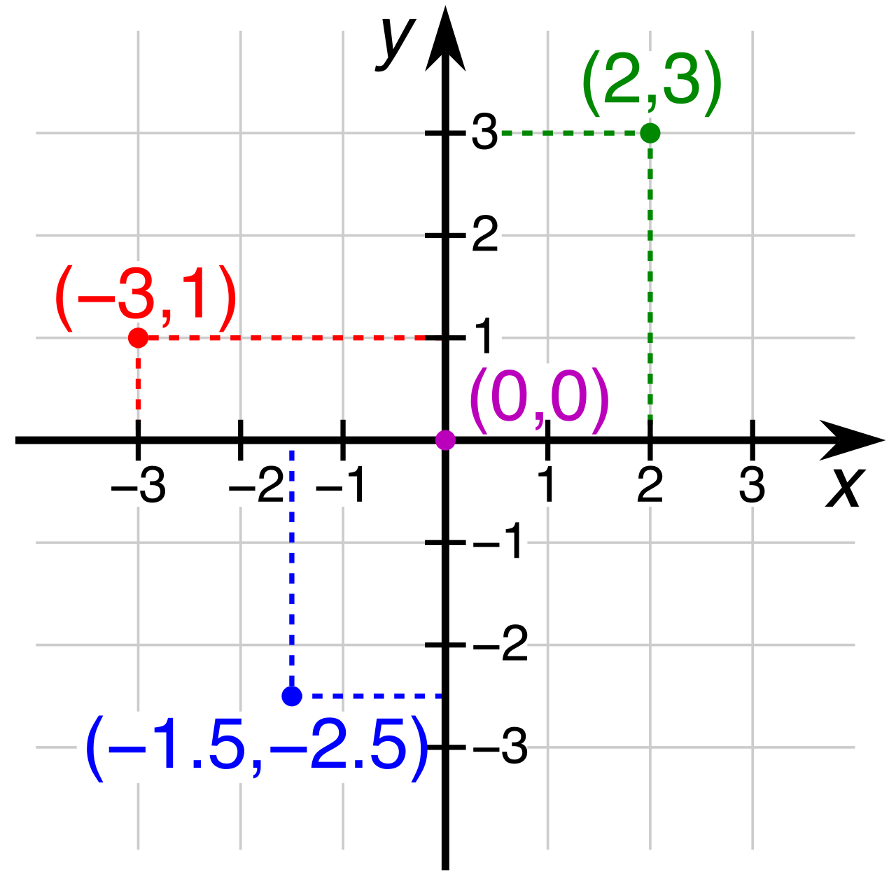
Consider the dashboard of a car accelerating onto a highway. The speedometer needle doesn’t merely display a number; its sweeping motion tells a physical story of force, mass, and time. When we graph a mathematical function, we are building a dashboard for a relationship. The Cartesian plane is not merely a grid of discrete pixels; it is a canvas where algebraic rules manifest as geometric realities. For a secondary mathematics teacher, the ability to read, sketch, and translate these visual narratives is paramount. You are not just teaching students to plot coordinates—you are teaching them to decode the behavior of dynamic systems. Whether an object is in freefall, a bacteria population is multiplying, or an investment is accruing compound interest, the shape of the curve reveals the fundamental nature of the phenomenon. To master this language, we must intimately understand the anatomy of functions, from their local turning points to their behavior at the edges of infinity.

The Cartesian coordinate plane acts as a visual canvas where algebraic relationships and dynamic systems can be plotted and analyzed.

Before we classify specific families of functions, we must define the vocabulary used to describe any curve's behavior. When your students look at a graph, they must learn to scan it from left to right, exactly as they would read a sentence in English.

As the input values (the $x$ -values) march steadily to the right, what is the output value (the $y$ -value) doing?

Strictly Increasing: A function is strictly increasing on an interval if the function value increases as the input value increases throughout the entire interval. The curve climbs.
Strictly Decreasing: A function is strictly decreasing on an interval if the function value decreases as the input value increases throughout the entire interval. The curve falls.

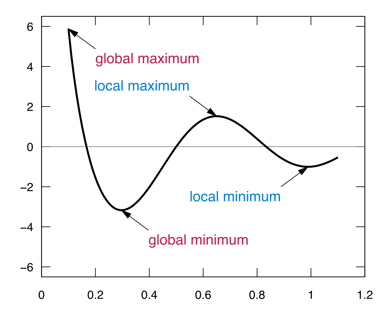
Where these intervals meet, the function changes direction. These transition points are the "peaks and valleys" of our graph, technically known as extrema.

Relative vs. Absolute Extrema

A relative maximum is a point on a graph where the function value is greater than or equal to the function values of all immediately adjacent points. It is a local hilltop.

A relative minimum is a point on a graph where the function value is less than or equal to the function values of all immediately adjacent points. It is a local valley.

An absolute maximum is the highest function value achieved over the entire specified domain of the function.

An absolute minimum is the lowest function value achieved over the entire specified domain of the function.

A visual representation distinguishing between relative extrema (local peaks and valleys) and absolute extrema (the highest and lowest overall points) on a defined interval.

A fundamental hurdle for students is confusing the value of the extremum (the $y$ -coordinate) with the location where it occurs (the $x$ -coordinate). If a quadratic function models the flight of a baseball, the absolute maximum is the peak height the ball reaches; the $x$ -value is merely the time it took to get there.

When translating a verbal description into a graph, the very first task requires accurately identifying the independent variable for the horizontal axis and the dependent variable for the vertical axis. Time, distance, or items produced typically drive the scenario (independent), while cost, height, or temperature respond (dependent).

Next, we establish our anchor. An initial starting value given in a verbal functional description directly corresponds to the y-intercept on the resulting plotted graph. This is the point where the graph of the function intersects the vertical axis, representing the state of our system at "time zero."

Once anchored, we analyze the rate of change:

A constant rate of change presented in a verbal scenario dictates the drawing of a straight linear segment on the corresponding graph.
A variable rate of change that continuously increases or decreases in a verbal scenario dictates the drawing of a curved non-linear segment on the corresponding graph.

If a student is modeling a leaky bucket that drips exactly $2$ milliliters per minute, they will draw a straight, descending line. If they are modeling a car aggressively braking, the velocity drops rapidly at first and then levels off—a curve.

Secondary mathematics curricula heavily rely on three core function families to model the world.

Linear Functions

The graph of a linear function is a straight line with a constant rate of change known as the slope. It is the geometry of steady, uniform progress. Whether you are paying a flat hourly rate for a plumber or traveling at cruise control, linear functions rule.

Quadratic Functions

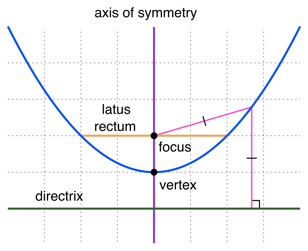
When the rate of change itself is changing at a constant rate (like the acceleration of gravity), we step into the second degree. The graph of a quadratic function is a symmetric U-shaped curve called a parabola.

Because of this symmetry, the vertex of a parabola represents the absolute maximum or absolute minimum of the corresponding quadratic function. Furthermore, the architecture of the parabola is perfectly balanced; the axis of symmetry of a quadratic function is a vertical line passing directly through the vertex of the parabola. If you know one side of the parabola, you know the other.

The anatomy of a parabola, illustrating its defining features including the vertex and the central axis of symmetry.

Exponential Functions

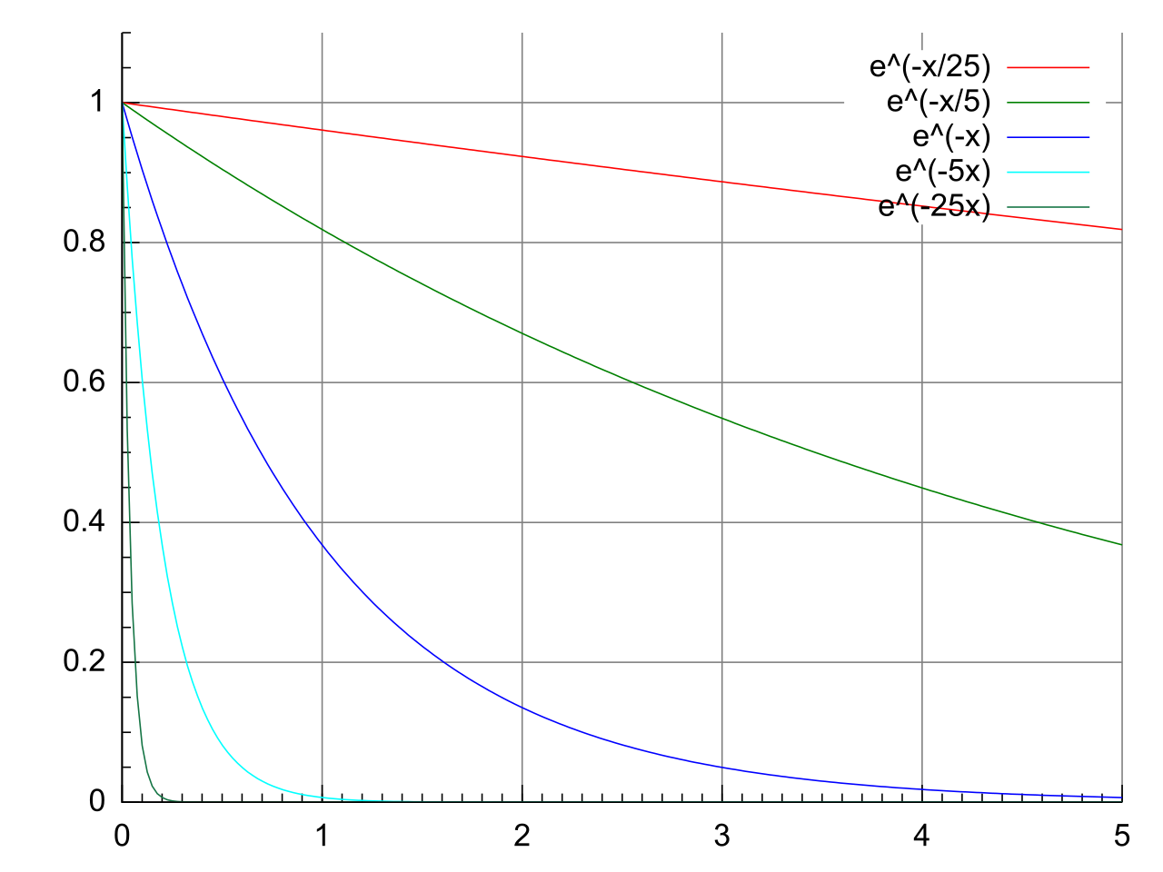
While linear functions add a constant amount over equal intervals, an exponential function models growth or decay with a constant multiplicative rate of change over equal intervals. Think of compound interest or radioactive half-life.

Exponential decay introduces a profound concept to students: limits. The graph of a basic exponential function possesses a horizontal asymptote representing a limit to the function's decay. Specifically, the horizontal asymptote of a basic exponential function of the form $y = a \cdot b^x$ is the line $y = zero$ . You can halve a piece of paper forever, and theoretically, it will never entirely disappear.

Graphs of varying exponential decay models demonstrating how the curve continually flattens as it approaches, but theoretically never reaches, the horizontal asymptote at y = 0.

When we expand beyond quadratics to higher-degree polynomials, the graphs become more dynamic.

Roots and the x-axis

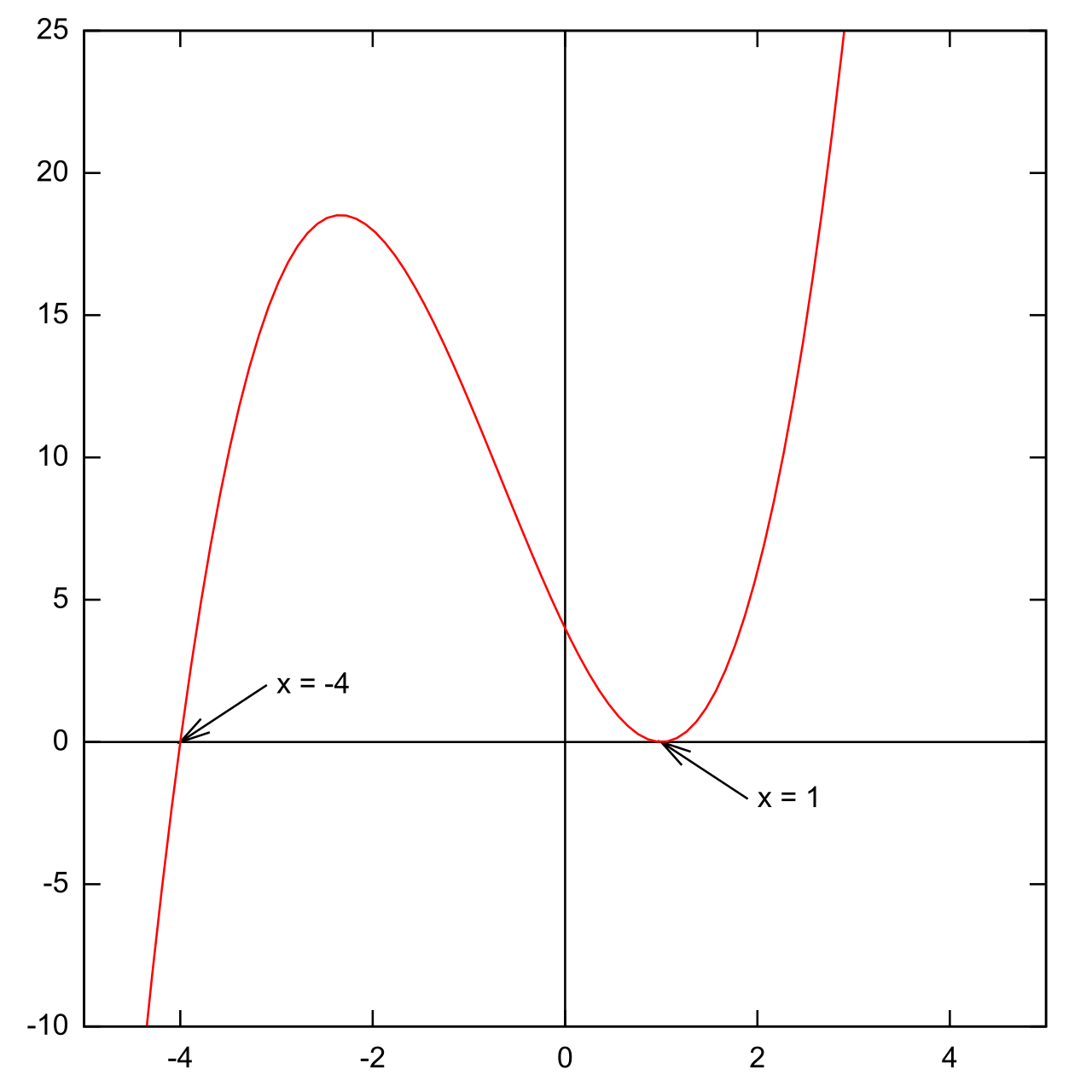
The x-intercepts of a polynomial graph represent the real roots or zeros of the polynomial function. But how the graph interacts with the $x$ -axis at these roots depends on the algebraic multiplicity of the factor.

Odd Multiplicity: A polynomial graph completely crosses the $x$ -axis at a root if the corresponding linear factor has an odd multiplicity (e.g., $(x-2)^1$ or $(x-2)^3$ ).
Even Multiplicity: A polynomial graph touches the $x$ -axis and turns around at a root if the corresponding linear factor has an even multiplicity (e.g., $(x-2)^2$ ). It acts like a ricochet.

A polynomial graph demonstrating the difference in algebraic multiplicity: odd multiplicity at x = -4 crosses the axis, while even multiplicity at x = 1 acts as a tangent, touching the axis and turning around.

Turning Points

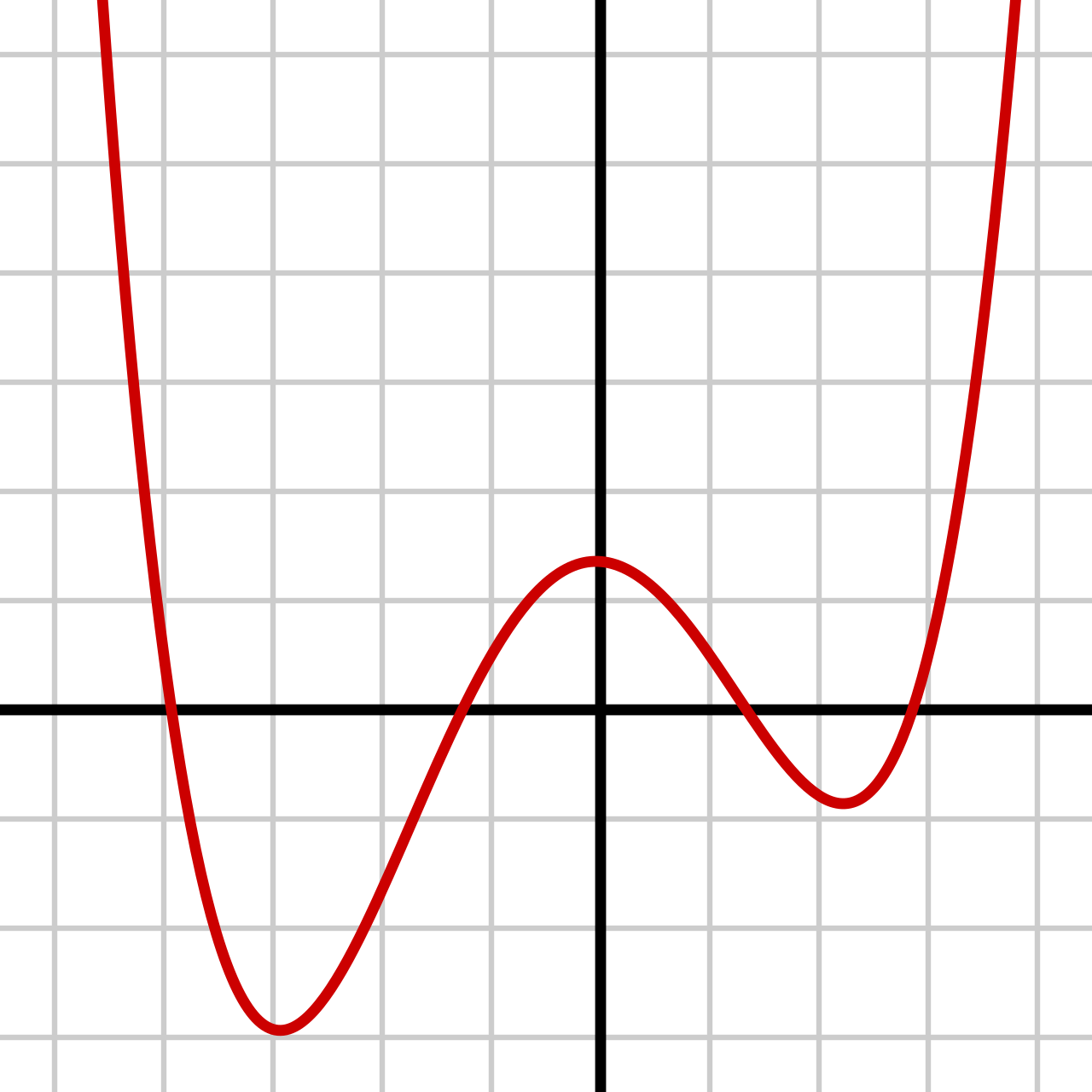
Between these roots, the polynomial must bend. The turning points of a polynomial graph correspond to the relative extrema of the polynomial function. The degree of the polynomial strictly limits its "flexibility." A polynomial function of degree $n$ can have at most $n - 1$ turning points. A cubic (degree 3) can turn at most twice; a quartic (degree 4) can turn at most three times.

End-Behavior

What happens when we zoom out to the edges of the Cartesian plane? End-behavior describes the trend of a function's output values as the input values approach positive infinity or negative infinity.

Because higher powers dominate massive numbers, the end-behavior of a polynomial function is determined entirely by the term with the highest degree. The rest of the terms represent mere statistical noise at infinity.

Degree	Leading Coefficient	End-Behavior (Left $\rightarrow$ Right)	Example Analogy
Even	Positive	Approaches positive infinity as the input approaches both positive and negative infinity.	Both arms raised in victory ( $+\infty$ , $+\infty$ ).
Even	Negative	Approaches negative infinity as the input approaches both positive and negative infinity.	Both arms pointing down to the floor ( $-\infty$ , $-\infty$ ).
Odd	Positive	Approaches negative infinity as input decreases, and positive infinity as input increases.	Uphill journey: falls left, rises right ( $-\infty$ , $+\infty$ ).
Odd	Negative	Approaches positive infinity as input decreases, and negative infinity as input increases.	Downhill journey: rises left, falls right ( $+\infty$ , $-\infty$ ).

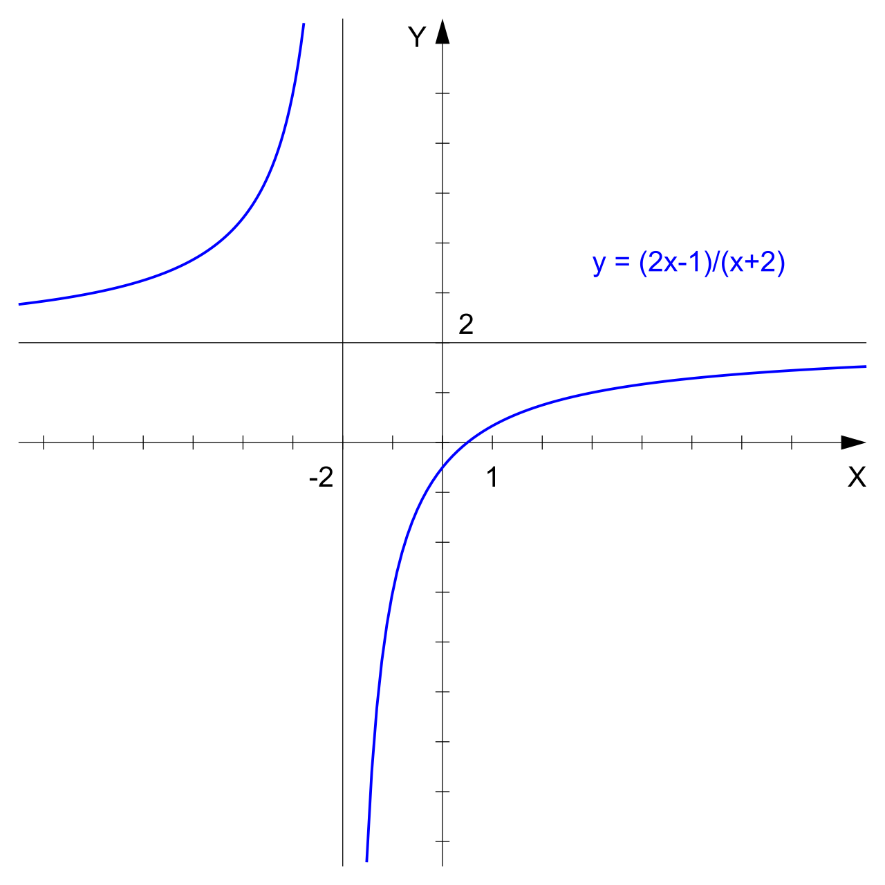
A rational function is defined as the quotient of two polynomial functions. Because division by zero is mathematically undefined, the denominator of a rational function acts as a strict boundary-setter, creating fractures in the graph.

Vertical Asymptotes and Holes

When a student looks at the denominator, they must ask: What $x$ -values break this machine?

A vertical asymptote occurs in the graph of a rational function at $x$ -values that make the denominator zero and the numerator non-zero. The function's output surges to infinity or plunges to negative infinity near this barrier.
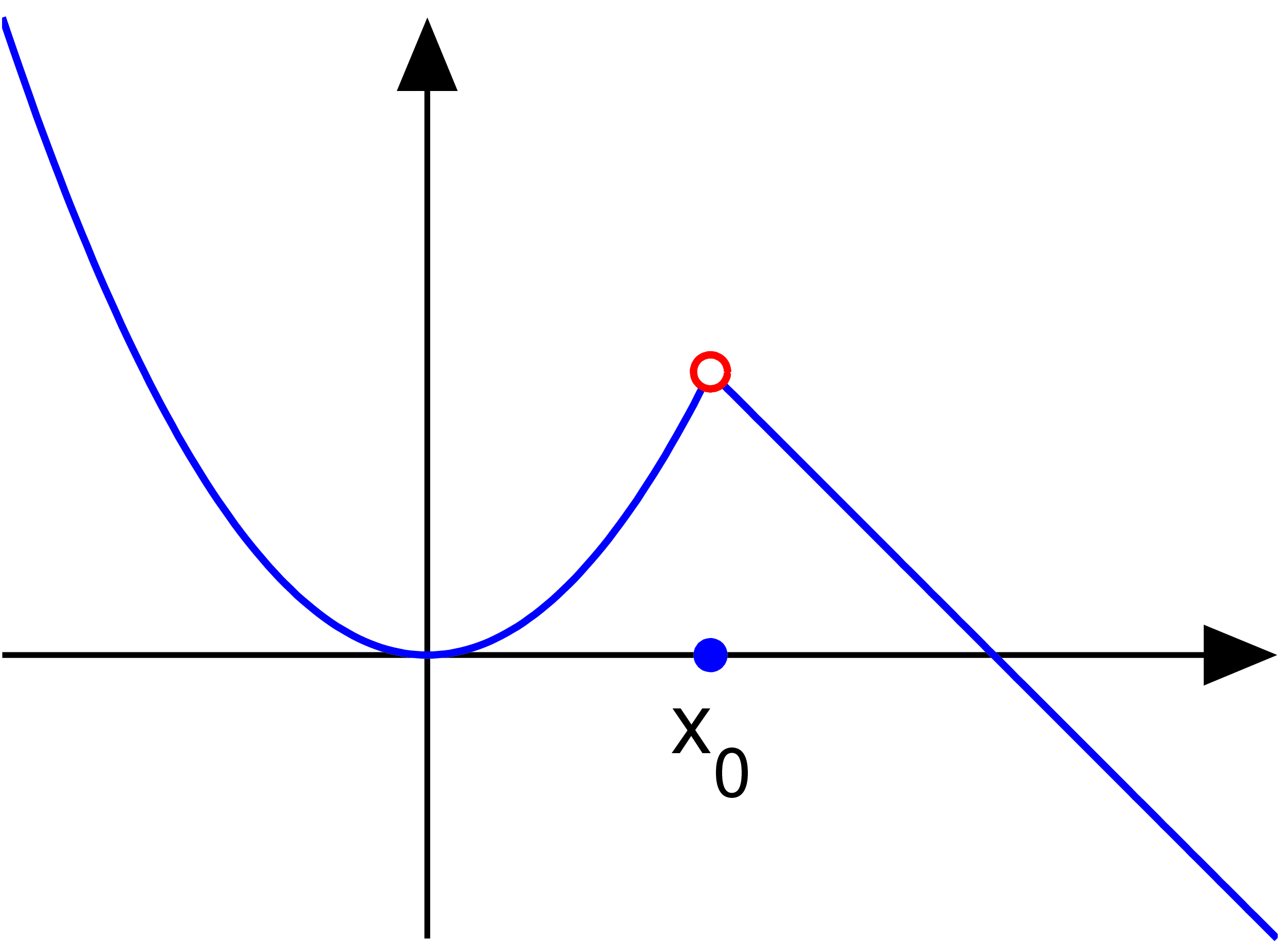
A hole or removable discontinuity occurs in the graph of a rational function when the numerator and denominator share a common linear factor. The graph looks continuous but is pierced by a single, infinitesimally small missing point.

A removable discontinuity, or 'hole', occurs at a specific x-value where the rational function is undefined, even though the surrounding curve appears continuous.

Horizontal and Slant Asymptotes

Just like polynomials, we must analyze the end-behavior of rational functions. A horizontal asymptote of a rational function indicates the end-behavior of the function as the input approaches positive or negative infinity. It is a tug-of-war between the degree of the numerator and the degree of the denominator.

Bottom-Heavy: A rational function has a horizontal asymptote at $y = zero$ if the degree of the numerator is strictly less than the degree of the denominator. The denominator overpowers the numerator, dragging the fraction toward zero.
Equally Weighted: A rational function has a horizontal asymptote equal to the ratio of the leading coefficients if the numerator degree is exactly equal to the denominator degree. They pull with equal force, settling into a stable horizontal limit.
Top-Heavy (by one): A slant or oblique asymptote occurs in a rational function graph when the degree of the numerator is exactly one greater than the degree of the denominator. As $x$ approaches infinity, the fraction behaves like a linear function.

The graph of a rational function fractured by a vertical asymptote where its denominator is zero, along with a horizontal asymptote that dictates its end-behavior.

Finally, we encounter functions that either change their rules midway or repeat their behavior endlessly.

Piecewise Functions

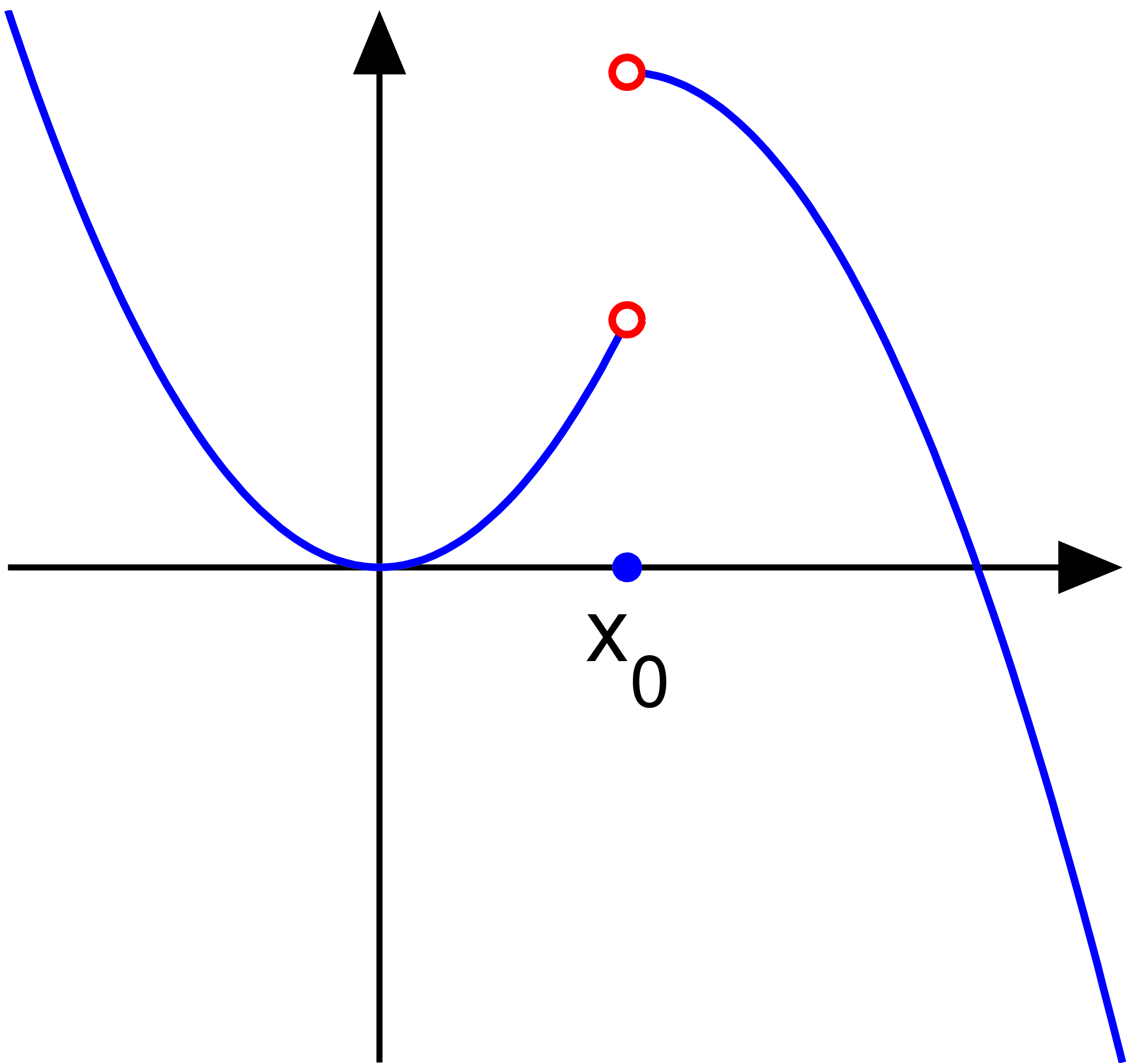
A piecewise function is defined by multiple sub-functions with each sub-function applying to a specific non-overlapping interval of the main function's domain. Consider tax brackets: your income up to $10,000 is taxed at one rate, and the income from $10,001 to $40,000 is taxed at another. The "rule" changes depending on where the input lands.

Because the rules change abruptly, a jump discontinuity frequently occurs in a piecewise function graph at the specific boundary points separating different sub-function domains. The graph literally leaps from one $y$ -value to another.

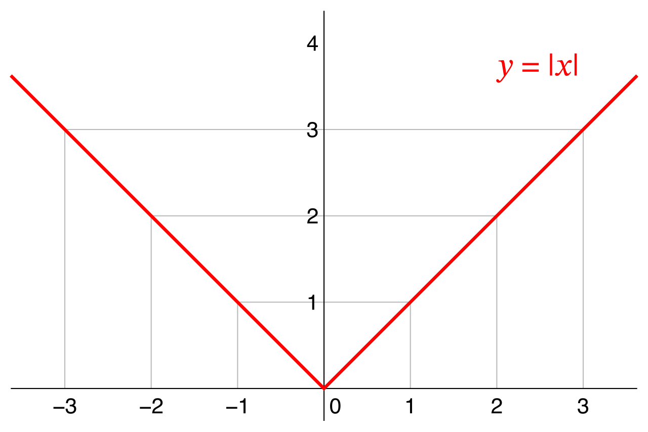
A jump discontinuity characteristic of piecewise functions, showing an abrupt leap between two different y-values as the domain rule changes.

A classic, ubiquitous example of piecewise logic is the absolute value function. The absolute value function can be graphically represented as a piecewise function consisting of two linear sub-functions meeting at a single vertex (forming a V-shape). For $x \ge 0$ , it behaves as $y=x$ ; for $x < 0$ , it behaves as $y=-x$ .

The absolute value function modeled as a piecewise graph, combining two linear sub-functions that converge at a central vertex.

Trigonometric Functions

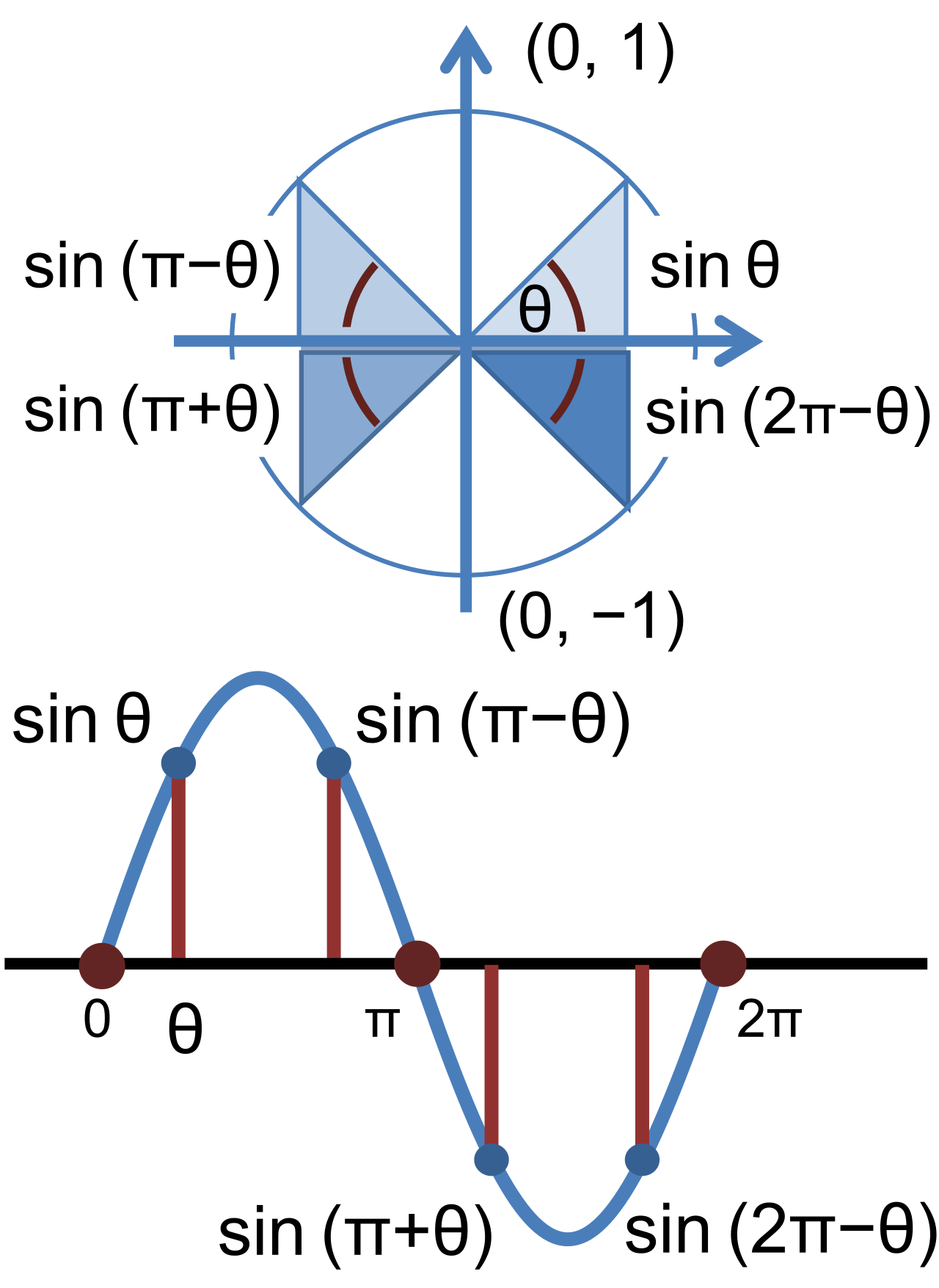
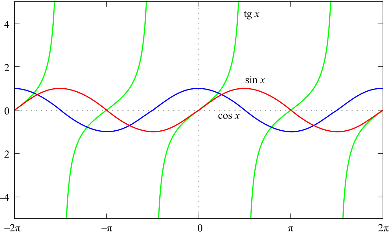
While polynomials stretch toward infinity, trigonometric functions oscillate. They are the geometry of the circle stretched out over time, perfectly suited to model pendulums, sound waves, and alternating current.

When analyzing a sinusoidal trigonometric function (sine and cosine), we look at four key features:

Amplitude: The amplitude of a sinusoidal trigonometric function is half the vertical distance between the absolute maximum and absolute minimum values. It measures the "loudness" or "intensity" of the wave.
Period: The period of a trigonometric function is the horizontal length of one complete non-repeating cycle of the function's graph.
Midline: The midline of a sinusoidal function is the horizontal line situated exactly halfway between the function's maximum and minimum vertical values. It represents the system's baseline resting state.
Phase Shift: A phase shift represents a horizontal translation applied to the graph of a trigonometric function, sliding the wave left or right along the $x$ -axis.

The sine function maps the vertical position of a point on a rotating unit circle over time, translating circular geometry into a continuous, oscillating wave.

While sine and cosine are smooth waves, their reciprocal and quotient counterparts are not. Because tangent, cotangent, secant, and cosecant involve division by sine or cosine, they inherit the fractures of rational functions. The graphs of the tangent, cotangent, secant, and cosecant functions contain infinitely many vertical asymptotes, occurring wherever their respective denominators equal zero.

Graphs of the sine, cosine, and tangent functions. The tangent graph features infinitely many vertical asymptotes occurring exactly where its denominator, the cosine function, equals zero.

Bringing It All Together

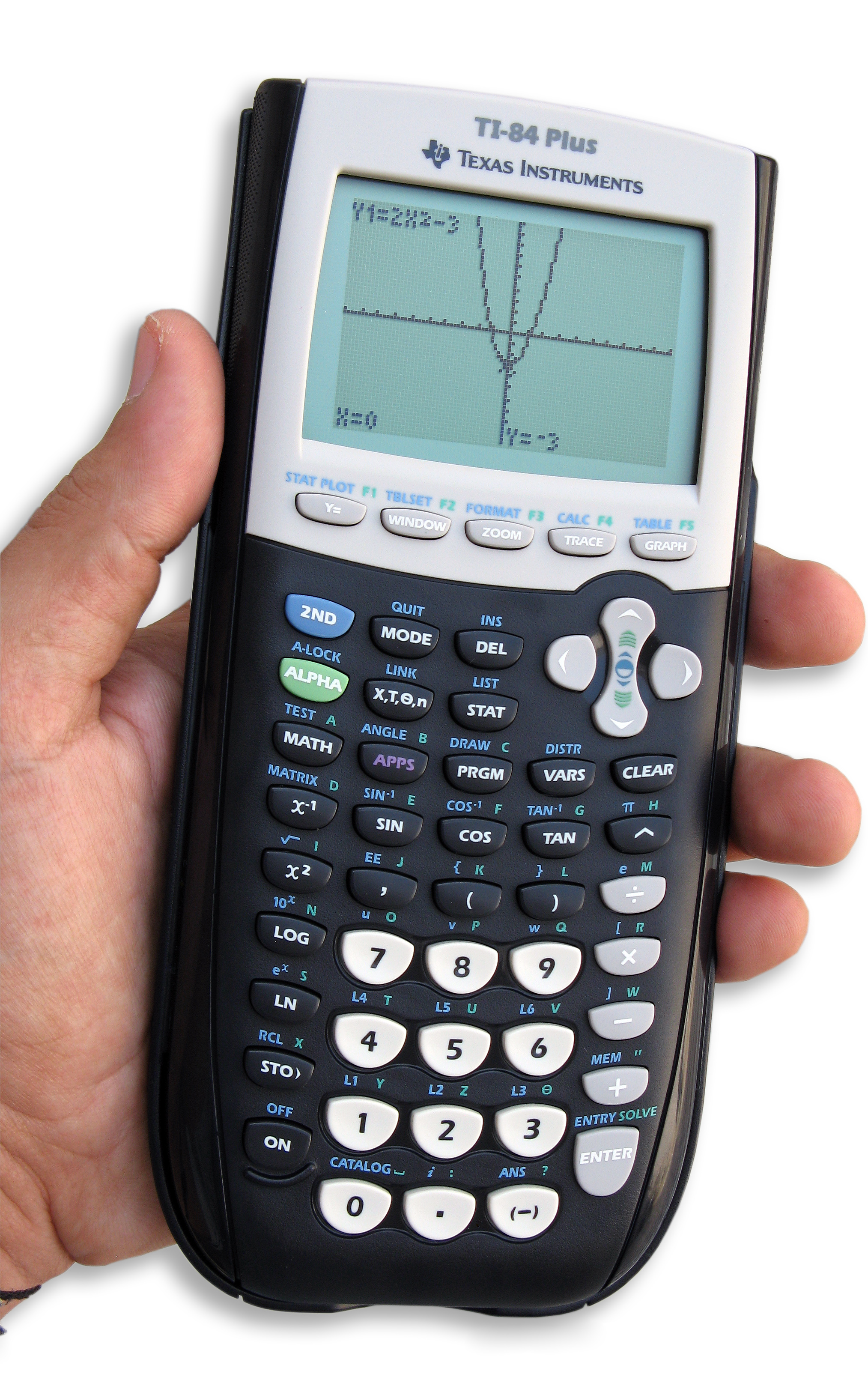
As you prepare to teach these concepts, remember that a graphing calculator is a tool for verification, not a substitute for intuition. By teaching your students to read intervals, spot extrema, respect asymptotes, and identify end-behavior, you empower them to predict what the screen will show before they ever press "GRAPH." You are teaching them to look at an equation and see the shape of reality hidden within it.

A graphing calculator provides visual verification, but true mathematical literacy requires the intuition to predict the graph's behavior before computing it.