Building and Transforming Functions
Not sure you’re ready?
Take the ~3-minute readiness diagnostic and see where you stand.
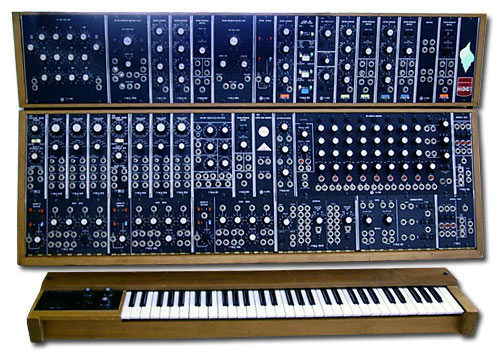
Imagine you are standing in front of a complex modular synthesizer, an interlocking system of cables, dials, and sound processors. You plug a raw audio signal into a filter—that is a mathematical function taking an input and producing an output. But the true power of this system does not emerge from a single, isolated filter. It emerges when you chain them together, route the output of an oscillator into a delay pedal, shift the pitch up by an octave, or reverse the waveform entirely. In the mathematics classroom, functions operate under the exact same paradigm. We rarely study functions in a vacuum; instead, we build new mathematical machinery through compositions, transformations, and inversions. For your future students, understanding how to manipulate these functions algebraically and graphically is the difference between blindly memorizing formulas and actually learning how to pilot the machinery of mathematics.
When your students manipulate functions on a graphing calculator, they often play a guessing game—blindly tweaking coefficients until a curve hits a desired target. As an educator, your goal is to transition them from guessing to engineering. Every analytical modification to a function's equation predictably dictates a geometric transformation of its graph.
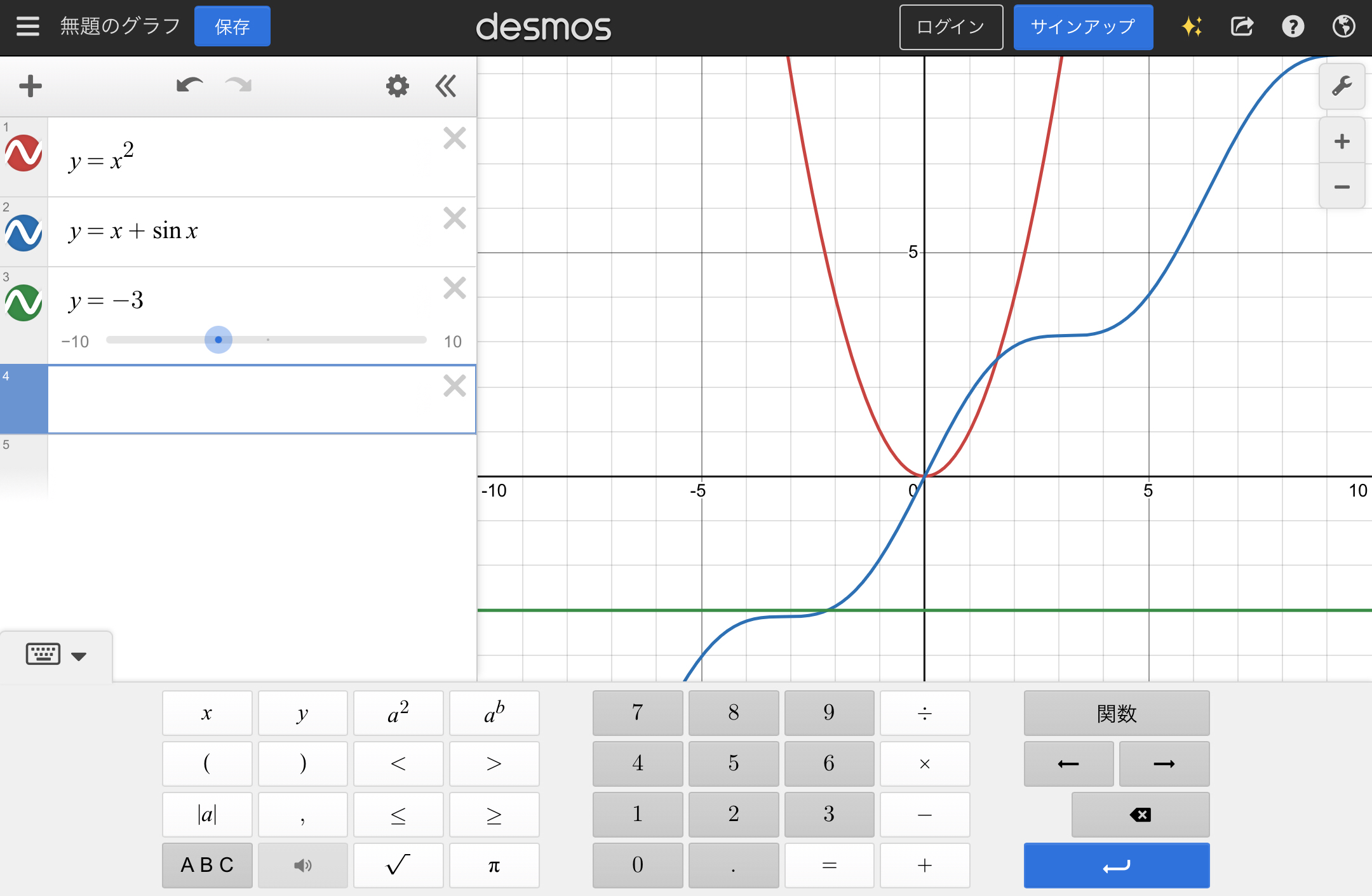
The most fundamental rule of function transformation is recognizing the boundary between the inside (the input) and the outside (the output) of the function.
Vertical Transformations (Modifying the Output)
Changes applied strictly to the output of f(x) affect the graph vertically, and they operate exactly as intuition suggests.
- Translations: Adding a positive constant k to a function's output to form f(x)+k translates the graph of the function vertically upward by k units. Conversely, subtracting a positive constant k from a function's output to form f(x)−k translates the graph of the function vertically downward by k units.
- Scaling: Multiplying a function's output by a constant a greater than 1 to form a⋅f(x) stretches the graph vertically by a factor of a. However, multiplying a function's output by a positive constant a less than 1 to form a⋅f(x) compresses the graph vertically by a factor of a.
- Reflections: Multiplying the output of a function by negative one to form −f(x) reflects the graph of the function across the x-axis.
Horizontal Transformations (Modifying the Input)
Changes applied directly to the independent variable x before the function acts upon it affect the graph horizontally. Students notoriously struggle here because the geometric effects appear to happen in reverse. You must explain why this happens: we are altering the timeline of the input.
- Translations: Subtracting a positive constant h from a function's input to form f(x−h) translates the graph of the function horizontally to the right by h units. (By subtracting, we delay the input; the function requires a larger x to achieve the original output). Conversely, adding a positive constant h to a function's input to form f(x+h) translates the graph of the function horizontally to the left by h units.
- Scaling: Multiplying a function's input by a constant b greater than 1 to form f(bx) compresses the graph horizontally by a factor of 1/b. We are feeding the function values at a faster rate, squishing the graph inward. Multiplying a function's input by a positive constant b less than 1 to form f(bx) stretches the graph horizontally by a factor of 1/b.
- Reflections: Multiplying the input of a function by negative one to form f(−x) reflects the graph of the function across the y-axis.
Order of Operations and The Factoring Trap
Transformations are not commutative. The sequence of applying transformations to a function matters and generally follows the order of operations from the inside of the function outward.
A critical pitfall arises when horizontal scaling and translations are combined. To correctly identify a horizontal shift when a horizontal compression or stretch is present, the expression inside the function must be factored into the form b(x−h).
The Factoring Warning: If a student looks at f(2x−6), they will often assume the graph shifts to the right by 6 units. By factoring the inner expression to f(2(x−3)), we reveal the true transformation: a horizontal compression by a factor of 1/2, followed by a horizontal shift right by only 3 units.
Certain transformations leave specific functions entirely unchanged. When reflecting a graph yields the exact same geometric figure, we have discovered an inherent symmetry.
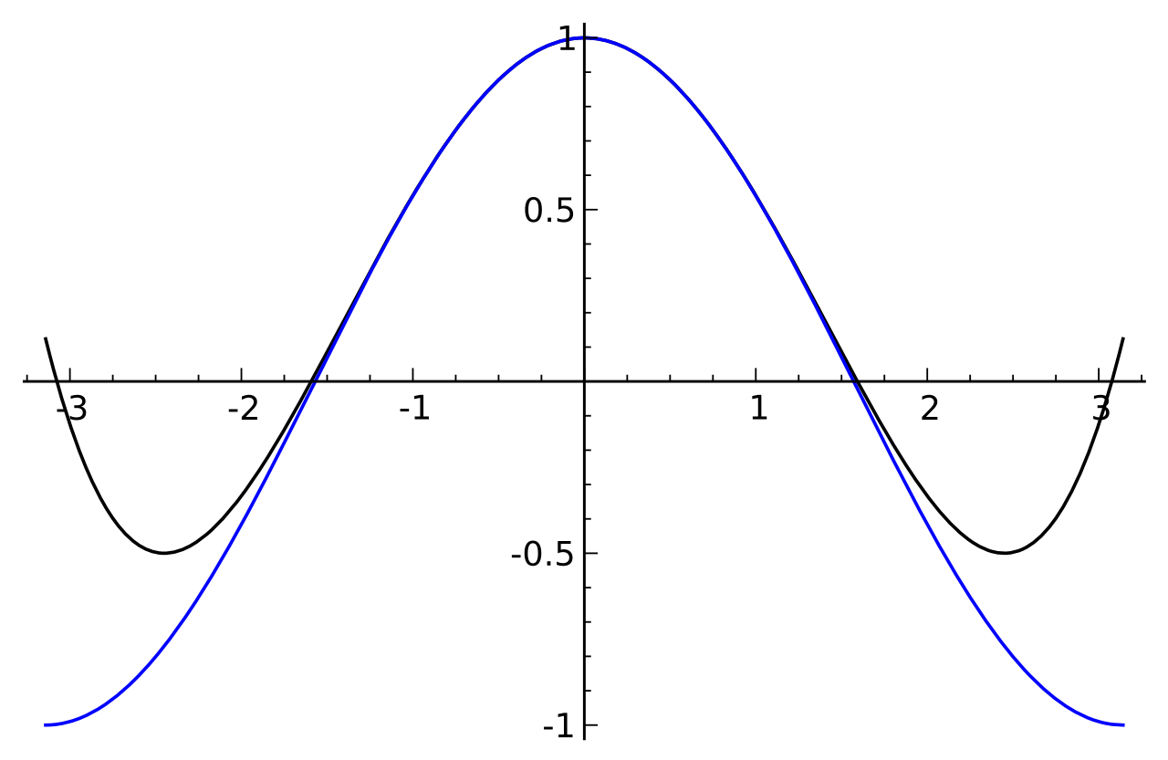
An even function satisfies the condition f(x)=f(−x) for all x in its domain. This means that negating the input produces no change in the output. Geometrically, the graph of an even function is structurally symmetric with respect to the y-axis.
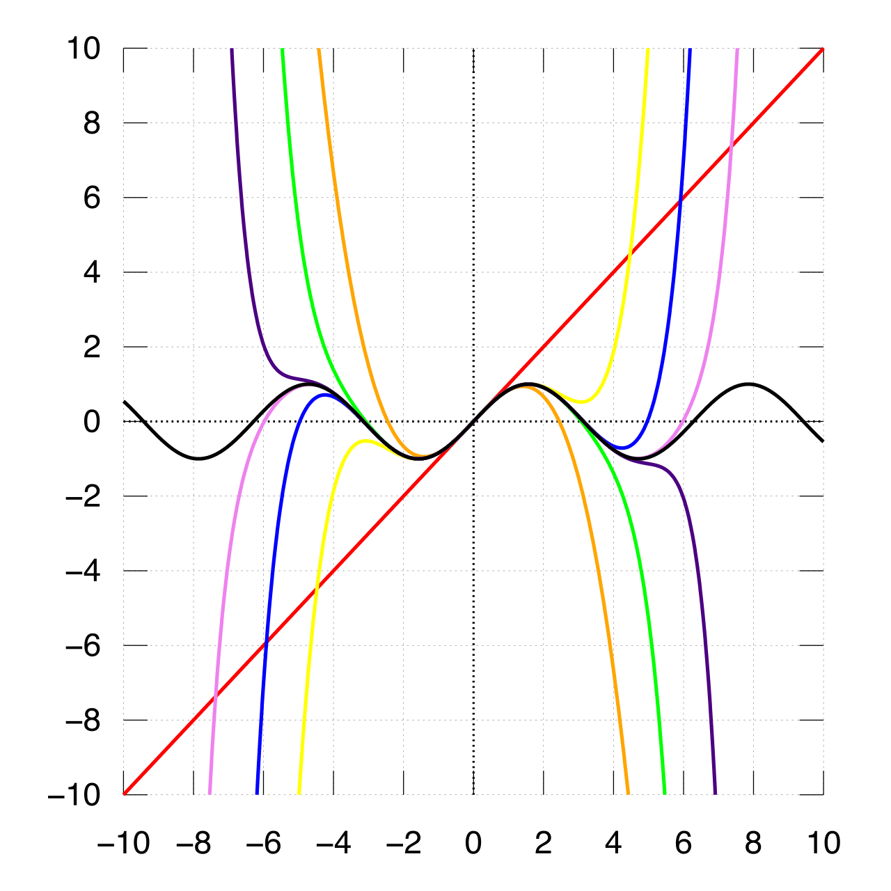
An odd function satisfies the condition f(−x)=−f(x) for all x in its domain. Negating the input perfectly negates the output. Because a horizontal reflection precisely matches a vertical reflection, the graph of an odd function is structurally symmetric with respect to the origin.
Just as numbers can be combined via fundamental arithmetic, so too can functions. However, combining functions requires strict bookkeeping of their domains. A combined function can only operate where all of its constituent parts are valid.
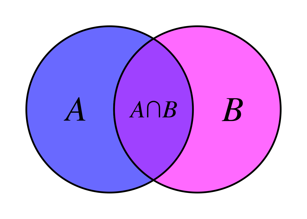
- Addition: The domain of the sum of two functions, denoted (f+g)(x), is the strict mathematical intersection of the domain of f(x) and the domain of g(x).
- Subtraction: The domain of the difference of two functions, denoted (f−g)(x), is the strict mathematical intersection of the domain of f(x) and the domain of g(x).
- Multiplication: The domain of the product of two functions, denoted (f⋅g)(x), is the strict mathematical intersection of the domain of f(x) and the domain of g(x).
- Division: The quotient introduces a new restriction. The domain of the quotient of two functions, denoted (f/g)(x), is the intersection of their individual domains excluding any x-values where g(x) equals zero.
The composition of two functions, denoted (f∘g)(x), requires evaluating the outer function f using the output of the inner function g(x) as its input. We are creating an assembly line where the raw material x is processed by g, and that finished product is immediately fed into f.
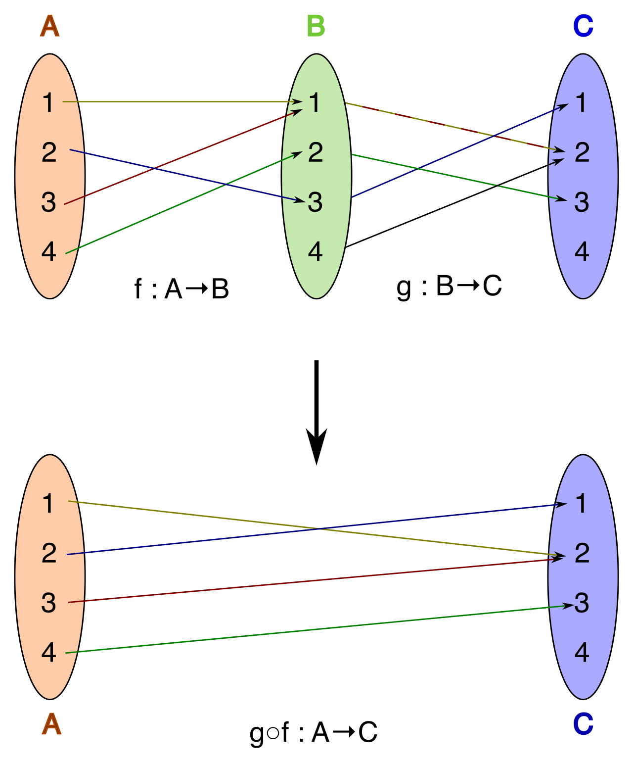
Because the order of the assembly line drastically alters the final product, function composition is not a commutative operation. Evaluating (f∘g)(x) is generally not equivalent to evaluating (g∘f)(x) for arbitrary functions. Putting on your socks and then your shoes yields a very different result than putting on your shoes and then your socks.
The Hidden Domain Restriction
When finding the domain of compositions, students frequently fall into an algebraic trap.
Crucial Rule: The domain of a composite function (f∘g)(x) consists only of x-values that are in the domain of g and for which g(x) is in the domain of f.
A composite function's domain must be analyzed before the final algebraic expression is completely simplified. Simplifying a composite algebraic expression can unintentionally hide domain restrictions originating from the inner function.
Consider f(x)=x2 and g(x)=x. The composition is (f∘g)(x)=(x)2=x. If a student only looks at the simplified result, y=x, they will mistakenly claim the domain is all real numbers. However, the inner function g(x) cannot process negative numbers. The machine broke at step one. Thus, the true domain of the composite function is restricted to x≥0.
If a function maps an input to an output, its inverse performs the exact opposite, retrieving the original input from the output. In a real-world scenario, if a function models cost based on item quantity, its inverse function models the item quantity based on a specific cost. This is immensely practical; a business owner does not just want to know how much 100 widgets will cost, but also how many widgets they can manufacture for $5,000.
To algebraicly prove two functions are inverses, we compose them. The composition of a function and its inverse yields the original input value for all values in the inverse's domain. The algebraic notation for the composition of a function f(x) and its inverse evaluated at x is f(f−1(x))=x.
The Precondition: One-to-One
Not every function can be reversed. A function must be strictly one-to-one to possess an inverse function over its entire domain. A function is one-to-one if each output value corresponds to exactly one unique input value.
Graphically, the horizontal line test determines whether a graphed function is one-to-one. If any horizontal line intersects a function's graph at more than one point, the function does not have a global inverse function. (If an output of y=4 maps back to both x=2 and x=−2, the inverse "machine" doesn't know which answer to output, violating the definition of a mathematical function).
Algebraic and Geometric Properties
Because the inverse swaps the roles of inputs and outputs, the domains and ranges are entirely exchanged:
- The domain of an inverse function is identical to the range of the original function.
- The range of an inverse function is identical to the domain of the original function.
To algebraically find the inverse of a function y=f(x), one swaps the x and y variables and solves the resulting equation for y.
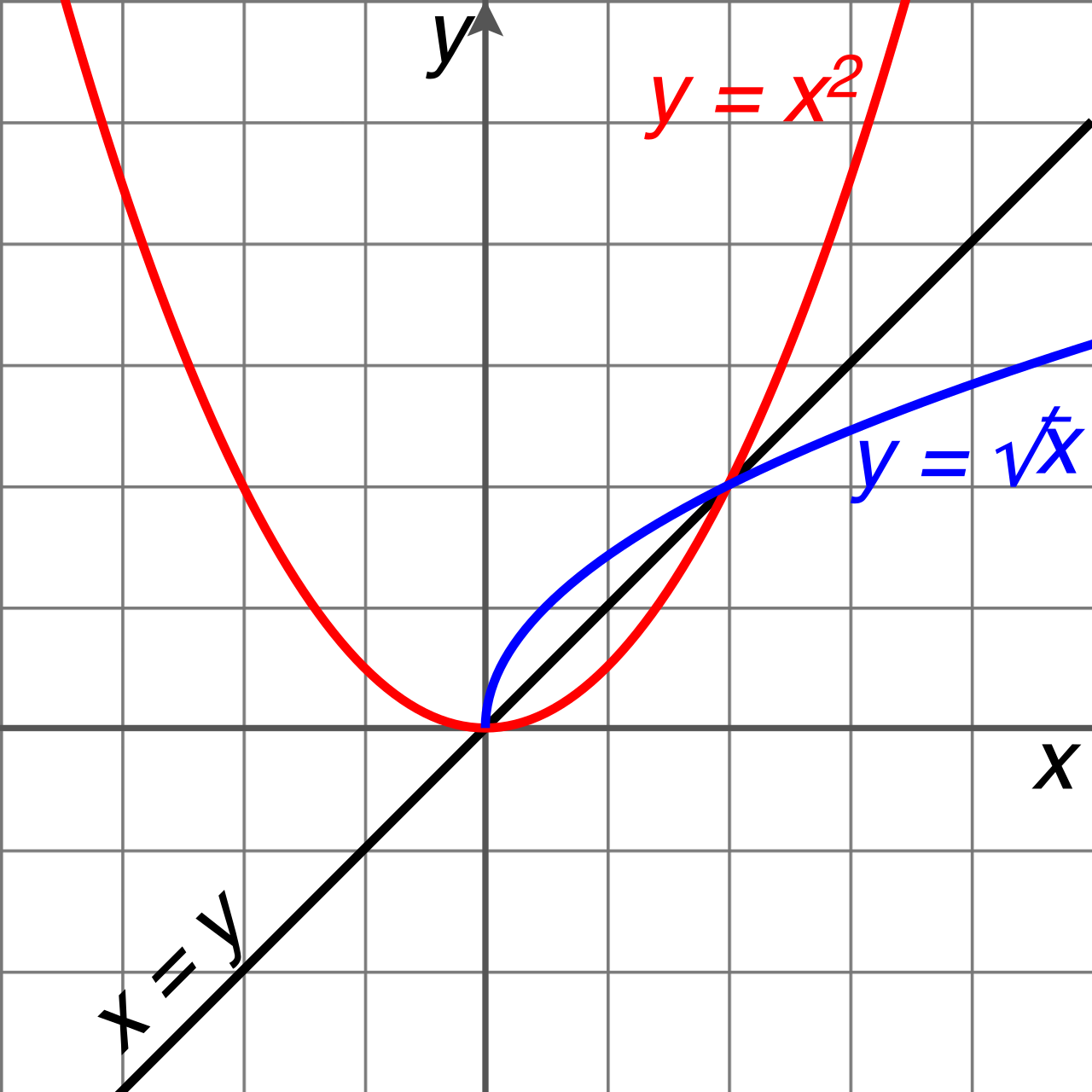
This algebraic variable-swap manifests beautifully in geometry. The graph of an inverse function is a geometric reflection of the original function's graph across the diagonal line y=x. Consequently, if a coordinate point (a,b) lies on the graph of a function, the coordinate point (b,a) lies on the graph of its inverse function.
Amputating the Domain
What happens when a highly useful function, like f(x)=x2, fails the horizontal line test? We force it to comply.
Restricting the domain of a non-one-to-one function allows an inverse function to be explicitly defined for that restricted domain. By discarding the problematic half of the graph, we create a purely one-to-one piece. Specifically, restricting the domain of the squaring function f(x)=x2 to x≥0 allows the creation of the principal square root inverse function, f−1(x)=x.
Understanding how to construct, manipulate, and dismantle functions empowers students to view mathematics not as a rigid set of rules, but as a flexible, logical toolkit. By mastering these transformations, domains, and inverses, you prepare your students to truly engineer their own mathematical solutions.