Analyzing Functions with Derivatives

Not sure you’re ready?

Take the ~3-minute readiness diagnostic and see where you stand.

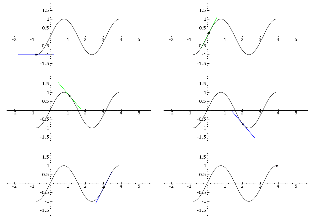
When a car navigates a winding mountain pass, its dashboard tells a continuous story of change. The speedometer captures the exact velocity at a frozen millisecond, while the altimeter tracks the sweeping changes in elevation. In calculus, derivatives provide this mathematical dashboard for any curve imaginable. The first derivative of a function represents the instantaneous rate of change of the function, capturing the exact trajectory of a curve at a single point. To analyze a function is to reverse-engineer its shape by reading this dashboard. For the secondary educator, mastering the translation between algebraic derivatives and geometric behavior is not merely about executing algorithms. It is about building the rigorous intuition necessary to teach a student how to visualize invisible rates of change.

To understand a function's behavior, we first look to its direction. The historical development of this concept gave us two distinct ways to write this down: the prime notation for derivatives ( $f'$ ), which was introduced by mathematician Joseph-Louis Lagrange, and the fractional notation ( $dy/dx$ ), which was created by mathematician Gottfried Wilhelm Leibniz. Regardless of the notation, the first derivative acts as a mathematical compass.

A manuscript by Gottfried Wilhelm Leibniz, whose development of calculus gave us the fractional notation (dy/dx) to describe instantaneous rates of change.

A function is strictly increasing on intervals where the first derivative of the function is positive ( $f'(x) > 0$ ), meaning the curve is rising. Conversely, a function is strictly decreasing on intervals where the first derivative of the function is negative ( $f'(x) < 0$ ), meaning the curve is falling.

To map these intervals seamlessly, we use a sign chart. A sign chart maps the positive and negative intervals of a derivative to systematically analyze the behavior of a function. The boundaries of these intervals are the points where the function momentarily pauses or breaks—these are our critical points.

Critical Points vs. Stationary Points

The distinction between a critical point and a stationary point is a common trap for students.

Stationary points are points on a graph where the first derivative is exactly zero.
Critical points encompass a broader category. Critical points of a function occur at domain values where the first derivative is exactly zero or where the first derivative is undefined.

Therefore, all stationary points are classified as critical points, but critical points where the derivative is undefined are not stationary points.

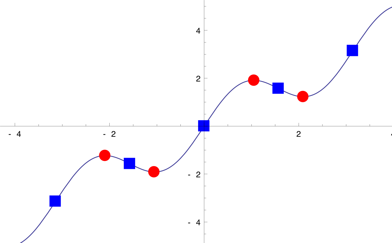
Stationary points (red circles) occur where the first derivative is zero, whereas inflection points (blue squares) occur where the second derivative changes sign.

Crucial Domain Check: A value must be in the domain of the original function to be classified as a critical point. If a rational function has a vertical asymptote at $x=2$ , the derivative will also be undefined there, but $x=2$ is not a critical point because the function does not exist there.

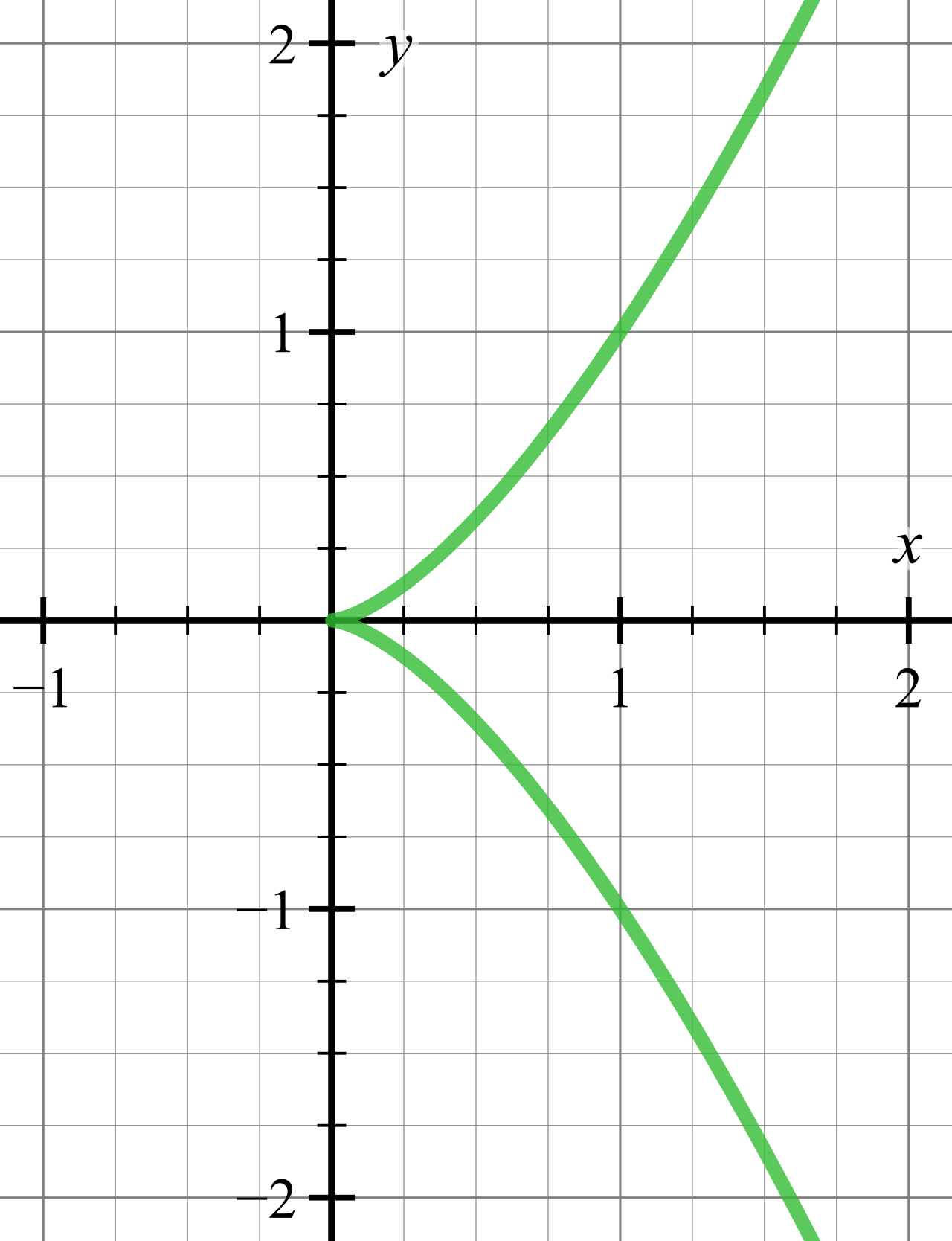
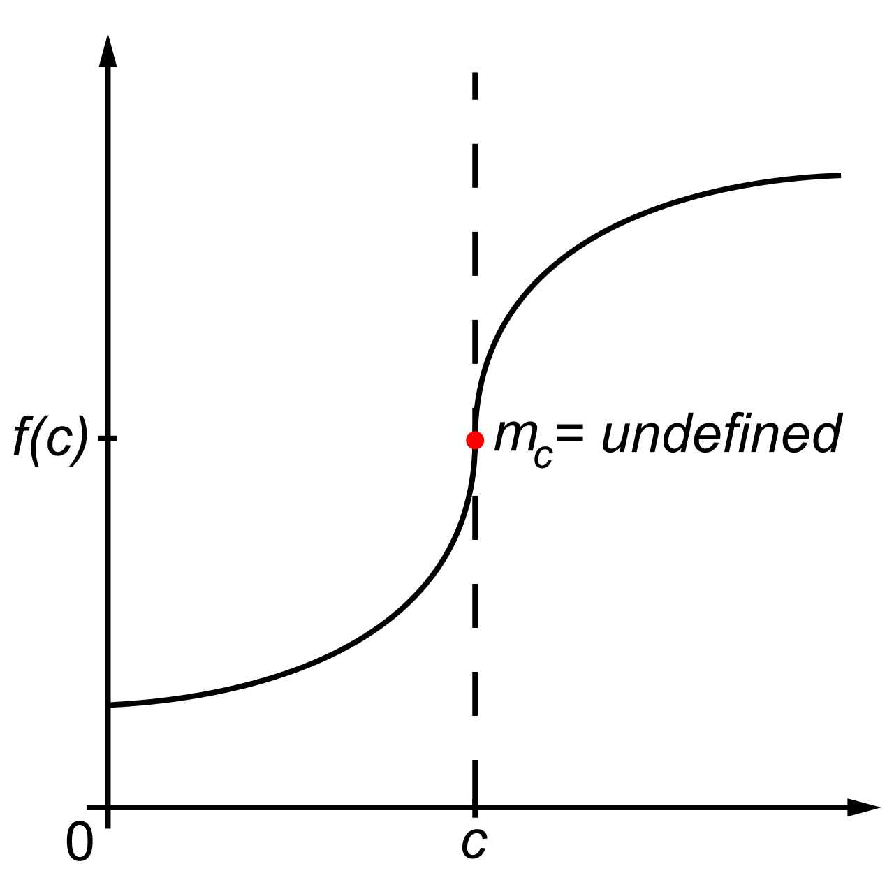
When the derivative is undefined at a valid domain value, it often manifests visually as a sharp turn or a vertical slope. For example:

Cusps represent domain values where the first derivative approaches positive infinity from one side and negative infinity from the other side (like the sharp point at the origin of $f(x) = x^{2/3}$ ).
Vertical tangents represent domain values where the first derivative approaches infinity from both sides (like the origin of $f(x) = x^{1/3}$ ).

A cusp manifests as a sharp point where the function is continuous, but the first derivative approaches opposite infinities from either side, rendering the derivative undefined.

A vertical tangent occurs when the first derivative approaches infinity from both sides, creating an undefined slope at a specific valid domain value.

Finding the Peaks and Valleys

Pierre de Fermat laid the groundwork for finding peaks and valleys when he developed Fermat's theorem on stationary points. Fermat's theorem states that local extrema of differentiable functions occur only at points where the derivative is zero.

Using our critical points, we can apply the First Derivative Test to classify these local extrema (note that relative extrema is a synonymous term for local extrema):

The First Derivative Test identifies a local maximum at a critical point if the first derivative changes from positive to negative at that point. (The function goes up, peaks, and comes down).
The First Derivative Test identifies a local minimum at a critical point if the first derivative changes from negative to positive at that point. (The function goes down, bottoms out, and comes up).

If the first derivative is the function's compass, the second derivative is its steering wheel. The second derivative of a function measures the rate of change of the first derivative. It tells us how the slope itself is changing. This concept is called concavity.

A function is concave up on intervals where the second derivative of the function is positive ( $f''(x) > 0$ ). The slopes are increasing (e.g., turning left while driving). The curve resembles a cup that can hold water.
A function is concave down on intervals where the second derivative of the function is negative ( $f''(x) < 0$ ). The slopes are decreasing (e.g., turning right while driving). The curve resembles an umbrella.

Points of Inflection

A point of inflection is a point on a curve where the concavity of the curve changes. At this exact boundary, the curve stops bending one way and starts bending the other.

An inflection point occurs exactly where a curve transitions between concave up (blue tangent lines) and concave down (green tangent lines).

Conditions for an Inflection Point:

At a point of inflection, the second derivative of the function must be zero or undefined.

A second derivative value of zero at a specific point does not guarantee the existence of an inflection point. Consider $f(x) = x^4$ . At $x=0$ , $f''(0) = 0$ , but the curve is concave up on both sides.

An inflection point only exists if the second derivative changes sign across that specific point.

A function must be continuous at a specific point to have a point of inflection at that location.

The Second Derivative Test

We can also use concavity to quickly classify stationary points without building a full first-derivative sign chart. This is the Second Derivative Test:

The Second Derivative Test states that a function has a local minimum at a stationary point if the second derivative is positive there. (A horizontal tangent on a concave-up interval means you must be at the bottom of the "cup").
The Second Derivative Test states that a function has a local maximum at a stationary point if the second derivative is negative there. (A horizontal tangent on a concave-down interval means you must be at the peak of the "umbrella").

However, the test has a blind spot. The Second Derivative Test is inconclusive at a critical point if the second derivative evaluates to zero at that point. When this happens, you cannot guess the behavior; when the Second Derivative Test is inconclusive, the First Derivative Test must be used to classify the critical point.

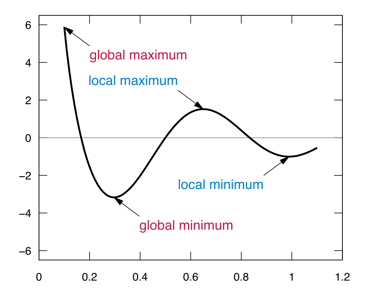
While local extrema tell us about the hills and valleys of a curve, we often need to find the absolute highest or lowest point overall. An absolute maximum is the highest value achieved by a function over its entire domain, and an absolute minimum is the lowest value achieved by a function over its entire domain. (Keep in mind, global extrema is a synonymous term for absolute extrema).

A graphical comparison of local extrema (relative peaks and valleys) and global extrema (the absolute highest and lowest points over the entire domain).

The Extreme Value Theorem (EVT)

When working on a restricted, closed interval $[a, b]$ , we rely on the Extreme Value Theorem, which guarantees both an absolute maximum and an absolute minimum for a continuous function on a closed interval.

The Extreme Value Theorem guarantees that any continuous function on a closed interval [a, b] will attain an absolute maximum (red) and an absolute minimum (blue).

To find these global peaks and valleys, we must check a specific list of suspects. Candidates for absolute extrema on a closed interval include all critical points within the interval, and equally importantly, candidates for absolute extrema on a closed interval include the endpoints of the interval. Evaluate the original function $f(x)$ at all critical points and endpoints; the highest resulting value is your absolute maximum, and the lowest is your absolute minimum.

The Mean Value Theorem and Rolle's Theorem

Derivatives also allow us to bridge the gap between average change and instantaneous change. The Mean Value Theorem states that for a continuous and differentiable function on a closed interval, there exists a point where the instantaneous rate of change equals the average rate of change. Geometrically, there is at least one point where the tangent line is perfectly parallel to the secant line connecting the endpoints.

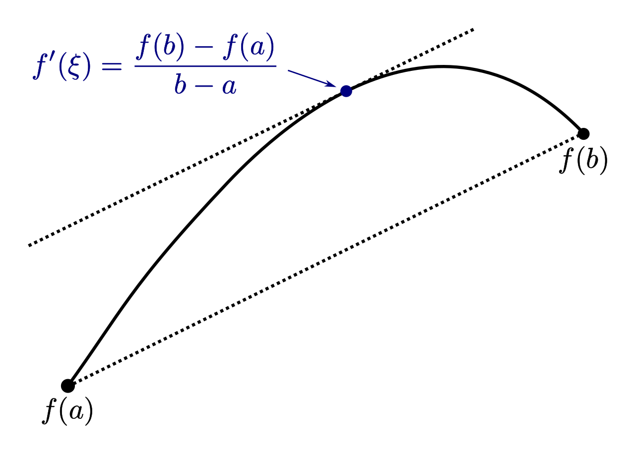
The Mean Value Theorem proves the existence of at least one point where the instantaneous rate of change (the tangent line) is perfectly parallel to the average rate of change (the secant line) between the interval's endpoints.

Rolle's Theorem is a special case of the Mean Value Theorem. If a secant line is perfectly horizontal, the average rate of change is zero. Therefore, Rolle's Theorem guarantees a point with a zero derivative between two points with equal function values for a smooth curve.

One of the most heavily tested skills on the Praxis 5165 exam—and a notorious hurdle for high school calculus students—is translating the graph of a first derivative, $f'$ , back to the original function, $f$ . You must divorce the y-values of the graph you are looking at from the shape of the graph you are looking at.

When you stare at a graph of $f'$ , read it using these precise rules:

On the graph of $f'$ ...	Translates to the behavior of $f$ ...
The x-intercepts of a first derivative graph...	...represent the critical points of the original function. (Because $f' = 0$ ).
Regions where the graph of the first derivative is above the x-axis...	...indicate where the original function is increasing. (Because $f' > 0$ ).
Regions where the graph of the first derivative is below the x-axis...	...indicate where the original function is decreasing. (Because $f' < 0$ ).
Intervals where a first derivative graph is increasing...	...correspond to intervals where the original function is concave up. (Because $f'' > 0$ ).
Intervals where a first derivative graph is decreasing...	...correspond to intervals where the original function is concave down. (Because $f'' < 0$ ).
The local maxima of a first derivative graph...	...correspond to points of inflection on the original function. (Because $f'$ changes from increasing to decreasing, meaning $f''$ changes from $+$ to $-$ ).
The local minima of a first derivative graph...	...correspond to points of inflection on the original function. (Because $f'$ changes from decreasing to increasing, meaning $f''$ changes from $-$ to $+$ ).

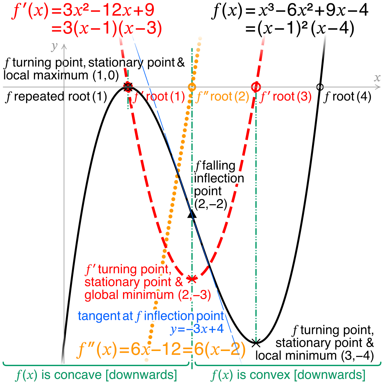
Analyzing a function through its derivatives: The original function (black) changes concavity at the exact point where its first derivative (red) reaches a local extremum and its second derivative (orange) crosses the x-axis.

When modeling this for your future students, always tell them to label the axes of a derivative graph with large $+$ and $-$ signs above and below the x-axis. It forces the brain to read the graph for value (positive/negative) rather than slope (rising/falling) when looking for the increasing/decreasing behavior of the original function.

Why do we care about mapping these peaks, valleys, and concavities? Because mathematics is the language of the physical universe.

Kinematics: The Physics of Motion

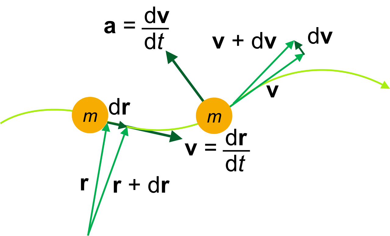
If we define a position function $s(t)$ that tracks an object over time, the derivatives give us the laws of motion:

The first derivative of a position function with respect to time represents instantaneous velocity. ( $v(t) = s'(t)$ )
The second derivative of a position function with respect to time represents instantaneous acceleration. ( $a(t) = v'(t) = s''(t)$ )

The kinematic relationship between a classical particle's position vector (r), its velocity vector (v, the first derivative), and its acceleration vector (a, the second derivative).

A classic conceptual pitfall occurs when analyzing the speed of a particle. Speed is the absolute value of velocity. An object can be moving backward (negative velocity) but speeding up (accelerating in that same negative direction).

The speed of a particle is increasing when its velocity and acceleration share the same mathematical sign. (Both positive, or both negative).
The speed of a particle is decreasing when its velocity and acceleration have opposite mathematical signs. (They are fighting each other).

Optimization

Finally, the most powerful application of extrema is optimizing systems to find the most efficient, cheapest, or largest possible outcome. Optimization problems use first and second derivatives to find the absolute maximum or absolute minimum of a contextual scenario.

Whether you are designing a cylindrical soup can to minimize aluminum cost (minimizing surface area given a fixed volume) or maximizing the area of a rectangular garden against a river with limited fencing, the mathematical process is identical:

Express the quantity to be optimized as a function of one variable.
Determine the physical domain boundaries of the scenario.
Find the critical points by setting the first derivative to zero.
Verify the absolute extrema using the First Derivative Test, Second Derivative Test, or by checking the closed-interval endpoints via the EVT.

By mastering how derivatives dissect a function, you are not just memorizing curve behaviors; you are learning how to rigorously optimize and predict the continuous changes of the real world.