Integration and Applications
Not sure you’re ready?
Take the ~3-minute readiness diagnostic and see where you stand.
Calculus concerns itself with two profound mathematical perspectives: shattering a continuous process into infinitesimal moments, and gathering those fragmented moments back into a cohesive whole. If differentiation is the mathematics of the shattered moment—capturing an instantaneous rate of change—then integration is the mathematics of accumulation. When we evaluate an integral, we are tallying up a continuous sweep of tiny changes to see the net result over space or time. The elongated 'S' symbol universally used to denote a mathematical integral was first introduced by Gottfried Wilhelm Leibniz precisely to represent this idea; it is simply an elongated "summa," the Latin word for sum. For an aspiring secondary mathematics teacher, mastering integration is not merely about algorithmic rule-following. It is about equipping your future students with the intellectual machinery to understand how velocity accumulates into distance, how bounding curves define regions of space, and how a sequence of discrete, rigid approximations seamlessly blurs into fluid, continuous reality.
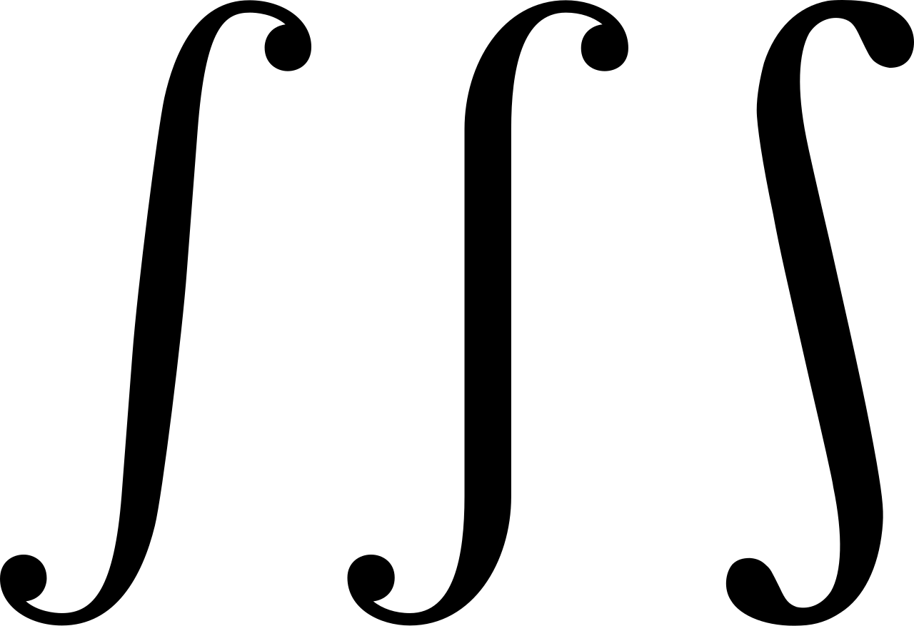
To teach integration effectively, you must delineate its two distinct personalities: the indefinite integral (a family of functions) and the definite integral (a specific numerical value representing accumulation).
The Indefinite Integral
When we speak of the indefinite integral, we are running the derivative machinery in reverse. The indefinite integral of a function represents the family of all possible antiderivatives of that function.
Because the derivative of any constant is zero, an infinite number of parallel functions share the same derivative. Consequently, every indefinite integral evaluation requires the inclusion of an arbitrary constant of integration—famously denoted as +C. To your students, forgetting the +C will seem like a trivial clerical error, but mathematically, omitting it denies the existence of the entire family of functions.
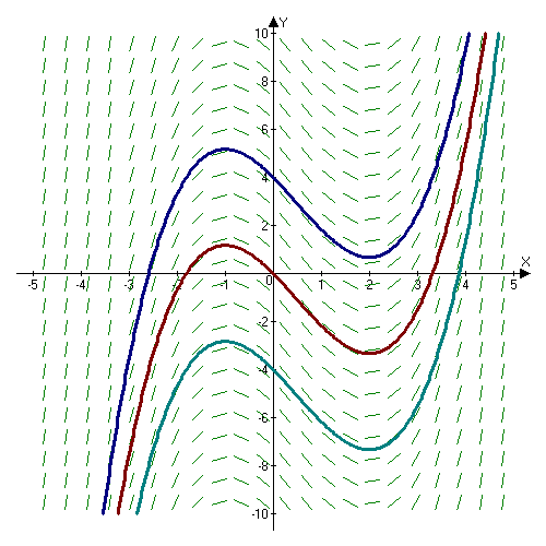
How do we single out one specific member of this family? Finding a specific continuous antiderivative from an indefinite integral requires an initial condition to solve for the constant of integration. If you know the starting value of a physical system—say, a particle's position at time t=0—you lock that floating family of curves into a single, concrete reality.
The Definite Integral
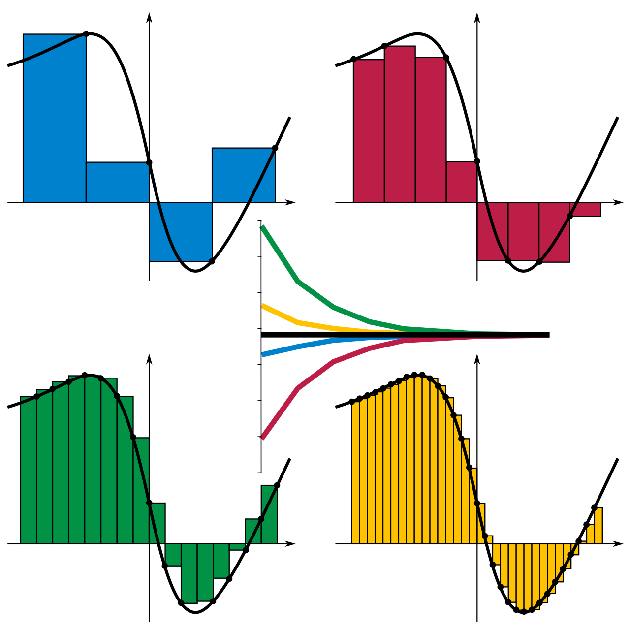
If indefinite integrals yield functions, definite integrals yield values. Imagine trying to find the area under a sweeping, curved archway. We cannot use standard geometry. Instead, we use a Riemann sum, which approximates the exact value of a definite integral by summing the areas of multiple rectangles inscribed beneath the curve.
As we make those rectangles infinitely thin, the jagged, stepped approximation becomes perfectly smooth. The definite integral of a continuous function represents the limit of its Riemann sums as the number of subintervals approaches infinity.
Before we apply calculus to the real world, we need a reliable toolkit. The fundamental techniques of integration mirror the rules of differentiation.
Standard Rules
- The Power Rule: Just as we multiply and subtract one from the exponent in differentiation, we do the reverse here. The power rule for integration states that the indefinite integral of x raised to the power of n is x raised to the power of n plus one, divided by n plus one (∫xndx=n+1xn+1+C).
- The Exception: The power rule for integration cannot be applied when the exponent of the variable is negative one (since dividing by −1+1 yields division by zero). Instead, the indefinite integral of the function one divided by x is the natural logarithm of the absolute value of x (∫x1dx=ln∣x∣+C). The absolute value is non-negotiable; logarithms cannot accept negative inputs, but 1/x operates perfectly fine in the negative domain.
- The Exponential: The easiest rule to memorize. The indefinite integral of the exponential function e raised to the x power is e raised to the x power. (∫exdx=ex+C).
- Trigonometric Functions:
- The indefinite integral of the sine function is the negative cosine function (∫sinxdx=−cosx+C).
- The indefinite integral of the cosine function is the positive sine function (∫cosxdx=sinx+C).
- Because the derivative of tangent is secant squared, the indefinite integral of secant squared of x is the tangent function of x (∫sec2xdx=tanx+C).
Reversing the Chain and Product Rules
When standard rules fail, we turn to structural reversals.
Integration by Substitution The method of integration by substitution reverses the chain rule process of differentiation. By identifying an inner function u and its derivative du sitting in the integrand, we collapse complex expressions into simple ones.
Crucial Trap for Students: When performing definite integration by substitution, the lower and upper limits of integration must be converted to correspond with the new substitution variable. If your students transition from x-space to u-space, they cannot evaluate the bounds using x-values unless they first translate the antiderivative back into terms of x. It is mathematically more elegant to simply change the bounds and finish the problem entirely in u-space.
Integration by Parts Integration by parts is an analytical integration technique derived from the product rule for differentiation. It is beautifully captured by the formula: the integration by parts formula states that the integral of u with respect to v equals the product of u and v minus the integral of v with respect to u. ∫udv=uv−∫vdu
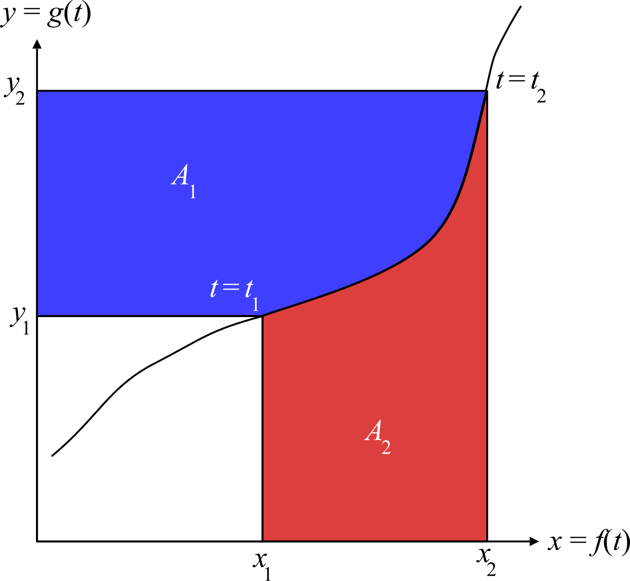
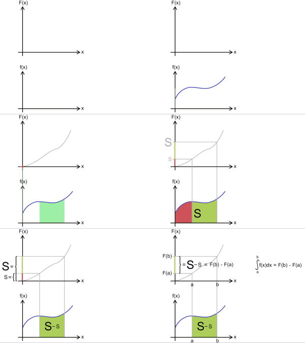
For much of mathematical history, finding tangent lines (derivatives) and finding areas (integrals) were completely distinct problems. The Fundamental Theorem of Calculus (FTC) is the spectacular realization that they are inverse operations.
The First Fundamental Theorem
The First Fundamental Theorem of Calculus establishes that the definite integral of a continuous function from a to b equals its antiderivative evaluated at b minus its antiderivative evaluated at a. ∫abf(x)dx=F(b)−F(a)
This theorem provides us with essential algebraic properties of the definite integral:
- The definite integral of any function evaluated from a lower limit of a to an upper limit of a is exactly zero. (An interval with no width contains no area).
- Reversing the upper and lower limits of a definite integral multiplies the original value of the integral by negative one. (∫baf(x)dx=−∫abf(x)dx). We are integrating "backwards" against the flow of the x-axis.
- The definite integral of a continuous function over adjacent intervals from a to b and from b to c equals the single definite integral from a to c.
We can also leverage geometric symmetry to bypass tedious algebra:
- The definite integral of an odd continuous function evaluated from negative a to positive a always equals zero. The area above the x-axis perfectly cancels the area below it.
- The definite integral of an even continuous function evaluated from negative a to positive a equals twice the integral of the function evaluated from zero to a.
The Second Fundamental Theorem
The Second Fundamental Theorem of Calculus states that the derivative with respect to x of a definite integral with a constant lower limit and variable upper limit x is the original integrand function evaluated at x. dxd(∫axf(t)dt)=f(x)
This mathematically formalizes the inverse relationship. However, if the upper limit is not simply x, the chain rule demands a toll. Applying the Second Fundamental Theorem of Calculus when the integral's upper limit is a composite function of x requires multiplying the evaluated integrand by the derivative of that upper limit.
Averages in Calculus
If a student scores 80,90, and 100 on three tests, they divide the sum by 3 to find an average. But how do we find the average temperature of a day when the temperature changes continuously every nanosecond?
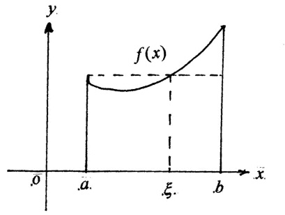
The average value of a continuous function on a closed interval is the definite integral of the function over that interval divided by the interval's width. favg=b−a1∫abf(x)dx
From this concept springs a profound guarantee: The Mean Value Theorem for Integrals guarantees that a continuous function on a closed interval will equal its average value at least once within that interval. If the average temperature over a 24-hour period was 70∘, at some specific, exact moment during the day, the thermometer read exactly 70∘.
One of the foundational uses of definite integrals in the secondary curriculum is calculating areas. We establish that the exact area bounded between a non-negative continuous curve and the x-axis is calculated using a definite integral.
But what if the region is floating in space, sandwiched between two curves?
| Orientation | Method of Calculation |
|---|---|
| Vertical Stacking (Functions of x) | The area of a two-dimensional region bounded by two functions of x is the definite integral of the upper boundary function minus the lower boundary function. (Top−Bottom) |
| Horizontal Stacking (Functions of y) | The area of a region bounded by two functions of y is calculated using the definite integral of the rightmost boundary function minus the leftmost boundary function. (Right−Left) |
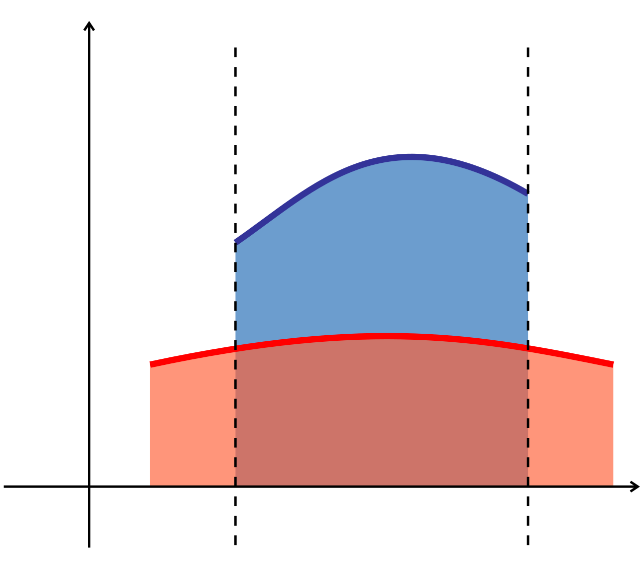
To evaluate these integrals (whether by hand or by inputting boundaries into a graphing calculator), we need specific intervals. The mathematical intersection points of two bounding curves establish the necessary limits of integration for calculating the area between them. You must set the two functions equal to each other to find where the "window" of area opens and closes.
Warning for students: Calculating the total area between two curves that cross each other requires splitting the definite integral at their intersection points. If Curve A is on top of Curve B, but then they cross and Curve B is on top, a single integral from start to finish will result in mathematical cancellation. Why does this matter? Because the calculated area between two or more geometric curves is always represented as a non-negative real number. There is no such thing as negative physical area in geometry.
If geometry is the spatial application of integration, kinematics is the temporal application. The relationships between position, velocity, and acceleration form a beautiful, real-world scaffolding for calculus.
When we move down the calculus ladder (differentiating), position becomes velocity, and velocity becomes acceleration. When we climb up the ladder (integrating), we reverse the flow:
- In kinematics, the velocity function of a moving object is the mathematical antiderivative of its acceleration function.
- The position function of a moving object in one-dimensional space is the mathematical antiderivative of its velocity function.
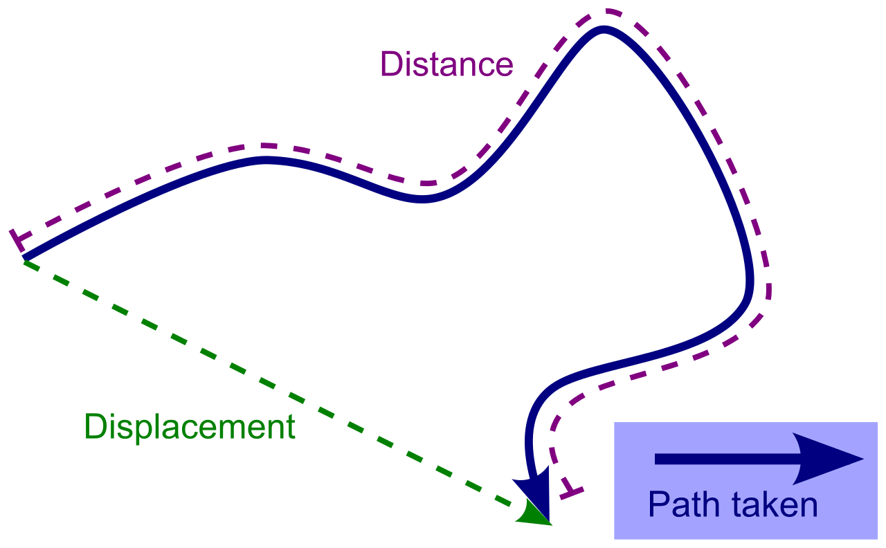
Displacement vs. Distance Traveled
This is a conceptual chokepoint for many students. Let's delineate them sharply:
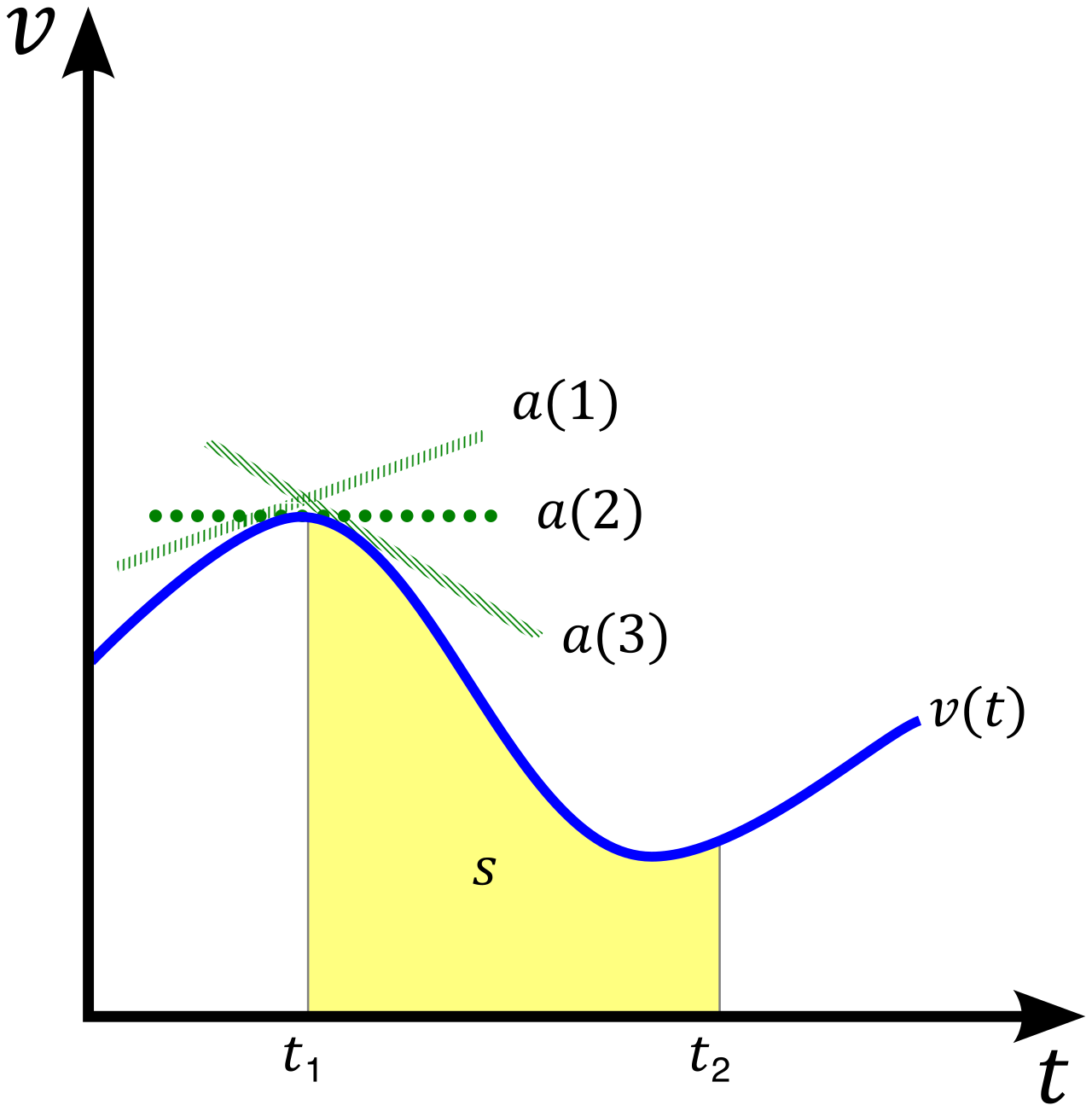
Displacement is simply where you end up relative to where you started. The displacement of an object over a specific time interval equals the definite integral of its velocity function over that time interval. Because moving backward cancels out moving forward, kinematic displacement indicates a net change in position and can result in a positive value, a negative value, or zero.
On the other hand, if you walk 5 miles east, and 5 miles west, your displacement is 0, but your pedometer reads 10 miles. Your pedometer measures total distance. The total distance traveled by an object equals the definite integral of the absolute value of its velocity function over a given time interval. Graphing calculators handle this elegantly: evaluating ∫∣v(t)∣dt will force all negative velocity (backward motion) to be tallied as positive distance.
Establishing Position and Speed
If we want to find the exact coordinates of an object at the end of a trip, displacement isn't enough; we need to know where we started. Therefore, the final spatial position of a moving object equals its initial position added to the definite integral of its velocity function. s(tfinal)=s(tinitial)+∫tinitialtfinalv(t)dt This is merely a rearrangement of the First Fundamental Theorem of Calculus, adapted for real-world utility!
Finally, how do we know if an object is actively speeding up or slowing down? Speed is the absolute value of velocity. An object speeds up when its velocity is pushed further away from zero.
- An object in rectilinear motion is considered to be speeding up when its velocity and acceleration functions share the same algebraic sign. (If you have negative velocity and negative acceleration, you are moving backward and being pushed harder backward—you are speeding up in reverse).
- An object in rectilinear motion is considered to be slowing down when its velocity and acceleration functions hold opposite algebraic signs. (If you are moving forward but the acceleration force is pushing backward, you are braking).
Concluding Note for the Educator
When you step in front of your classroom, your objective is to demystify the abstract. The definite integral is not just a limit of Riemann sums; it is the total distance shown on a car's odometer. The +C in an indefinite integral is not a pesky penalty point; it is the unknown starting coordinate of a GPS system. Master these nuances, clearly distinguish between your boundaries and conditions, and you will transform calculus from a collection of rote formulas into a dynamic language that describes the very fabric of reality.