Arithmetic and Geometric Sequences

Not sure you’re ready?

Take the ~3-minute readiness diagnostic and see where you stand.

Nature behaves in both continuous sweeps and discrete jumps. When a physicist models the trajectory of a thrown ball, they use a continuous curve because the ball occupies every infinitesimally small point in space along its path. However, when a school board allocates funding based on yearly enrollment, or a bank computes interest at the end of a month, the timeline fractures into distinct, countable steps. In mathematics, a sequence is a mathematical function whose domain is a subset of integers. More specifically, to align with the act of counting events or steps, the domain of a mathematical sequence is typically restricted to positive integers.

When we introduce sequence notation, the variable $n$ is not merely an arbitrary placeholder like $x$ in a continuous equation; the variable $n$ in sequence formulas represents the ordinal position of the term—the first term, the second term, the third, and so on. Because it denotes a discrete position, the sequence position variable $n$ must be an integer. As a secondary mathematics teacher, your task is to help students bridge their understanding of continuous functions (lines and curves drawn without lifting the pencil) to these discrete, stepwise realities.

Sequences operate on a discrete domain of positive integers, which can be visualized as distinct, countable points on a number line rather than a continuous span.

To describe a sequence mathematically, we have two distinct languages at our disposal: recursive and explicit. They are fundamentally different ways of answering the question, "What is the next number?"

A recursive formula calculates the $n$ th term of a sequence based on one or more previous terms in the sequence.

Think of a recursive formula as a set of walking instructions. If you want to know where you will be after ten steps, you must physically take step one, then step two, then step three. Because a recursive formula relies entirely on relative positioning, a recursive formula for a sequence must explicitly state at least one initial term to be completely defined. Without an initial term, you have instructions for taking a step, but no starting location.

An explicit formula calculates the $n$ th term of a sequence using only the position number $n$ .

If recursive formulas are walking instructions, explicit formulas are a teleportation machine. You input the destination coordinates ( $n$ ), and you arrive immediately. Whether you are dealing with arithmetic or geometric patterns, an arithmetic sequence can be evaluated for any term directly using the explicit formula without calculating preceding terms. The exact same advantage holds true for multipliers: a geometric sequence can be evaluated for any term directly using the explicit formula without calculating preceding terms.

Imagine a subway train that boards $15$ new passengers at every single stop. This perfectly illustrates an arithmetic progression. An arithmetic sequence is a sequence of numbers in which the difference between any two consecutive terms is a constant.

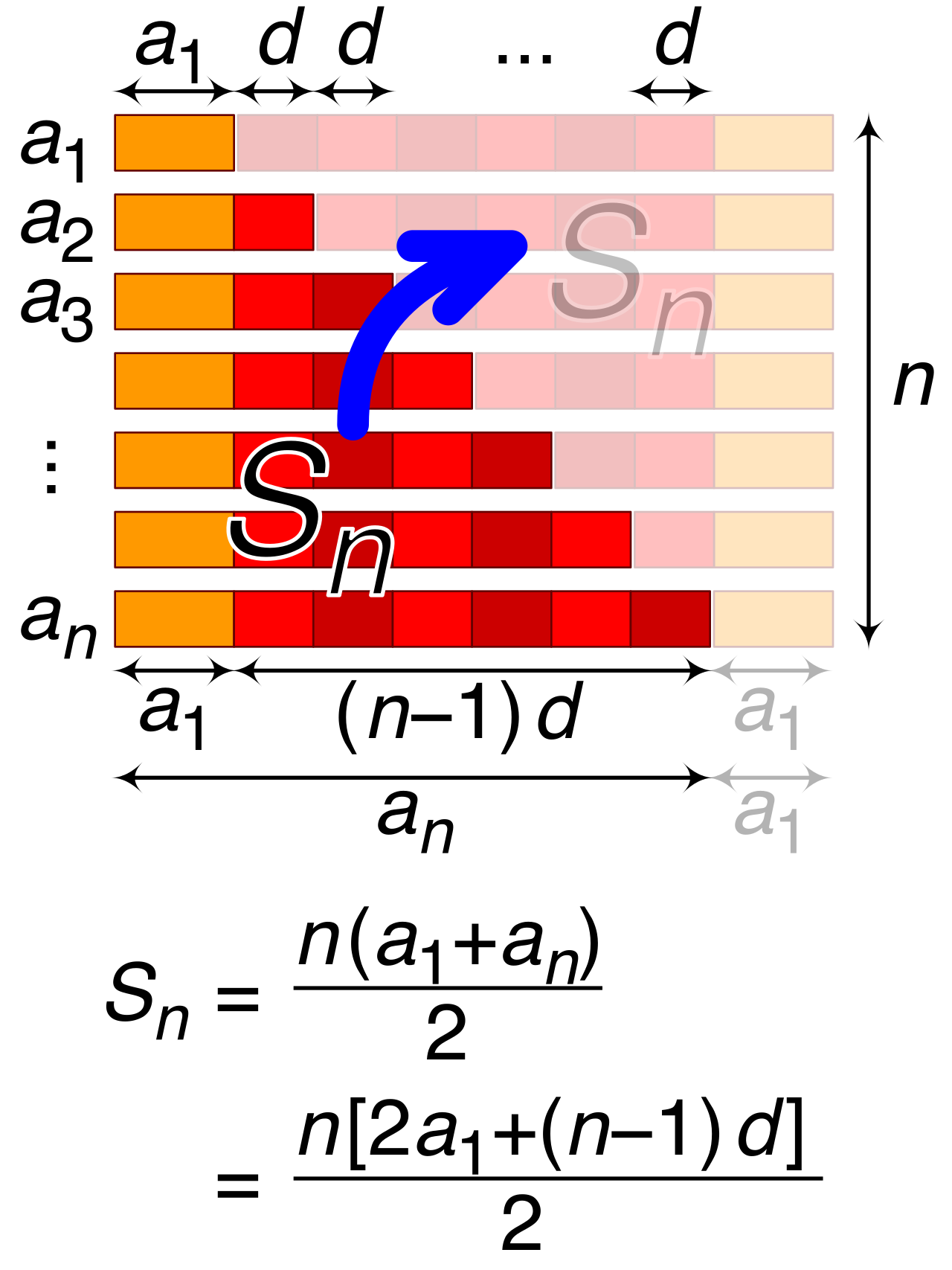
The constant difference between consecutive terms in an arithmetic sequence is called the common difference, typically denoted by $d$ . To find this value from a list of numbers, the common difference of an arithmetic sequence is calculated by subtracting a term from the immediately following term ( $d = a_n - a_{n-1}$ ).

A visual representation of an arithmetic progression, where each step increases by a constant common difference, akin to stacking an identical number of blocks in each successive column.

Formulas and Structure

The recursive formula for an arithmetic sequence is $a_n = a_{n-1} + d$ . It simply states: "To get the current term, take the previous term and add $d$ ."

However, if we want to bypass the stepping-stones, we need the explicit form.

The explicit formula for an arithmetic sequence is $a_n = a_1 + (n-1)d$ .

In this formula:

In the explicit arithmetic formula $a_n = a_1 + (n-1)d$ , the variable $a_1$ represents the first term.
In the explicit arithmetic formula $a_n = a_1 + (n-1)d$ , the variable $d$ represents the common difference.

Why $(n-1)$ ? This is a critical concept for students to grasp. If you want to arrive at the $5$ th term, you start at the $1$ st term and make exactly $4$ "jumps" of size $d$ . You always make one fewer jump than your destination's position number.

Modeling and Graphing

Because an arithmetic sequence changes by a fixed amount at each step, arithmetic sequences model linear growth or linear decay over discrete intervals. If you were to plot the values on a coordinate plane, an arithmetic sequence generates a linear graph when the sequence values are plotted against the term position numbers.

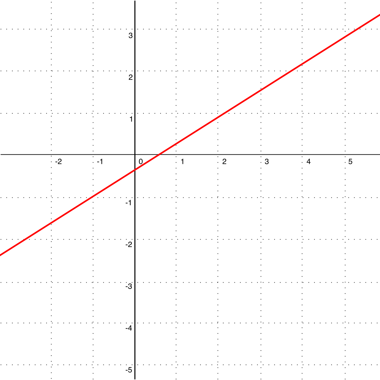
When plotted, the discrete terms of an arithmetic sequence align to form a linear graph, where the common difference functions geometrically as the slope of the line.

The algebraic connection here is profound. If you expand the explicit formula $a_n = a_1 + dn - d$ , and rearrange it to $a_n = d(n) + (a_1 - d)$ , it perfectly mirrors the slope-intercept form $y = mx + b$ . Therefore, in an arithmetic sequence, the constant rate of change is equivalent to the slope of a linear function.

In the real world, this behavior governs many linear financial and physical systems:

Real-world scenarios involving simple interest accumulation can be modeled using arithmetic sequences. If you invest $1,000 at $5\%$ simple interest, you earn exactly $50 every single year. The balance sequence ($1,050, $1,100, $1,150...) is arithmetic because the addition is constant.
More broadly, real-world scenarios involving a constant addition or subtraction of items over discrete steps can be modeled using arithmetic sequences, such as a reservoir draining at a steady 500 gallons per hour.

Now, imagine a scenario where a bacteria culture doubles every hour. The growth is no longer a steady addition; it is a steady multiplication. A geometric sequence is a sequence of numbers in which the ratio of any term to the preceding term is a constant.

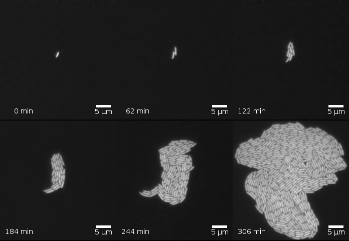
Bacterial colonies multiplying under optimal conditions provide a real-world model of a geometric sequence, where each time interval results in scaling by a constant ratio.

The constant ratio between consecutive terms in a geometric sequence is called the common ratio, denoted by $r$ . To identify this multiplier empirically, the common ratio of a geometric sequence is calculated by dividing a term by the immediately preceding term ( $r = \frac{a_n}{a_{n-1}}$ ).

Formulas and Structure

The recursive formula for a geometric sequence is $a_n = r \cdot a_{n-1}$ . The instruction is simple: "Multiply the previous term by $r$ ."

To jump directly to the $n$ th hour of bacterial growth, we use the explicit form.

The explicit formula for a geometric sequence is $a_n = a_1 \cdot r^{n-1}$ .

In this formula:

In the explicit geometric formula $a_n = a_1 \cdot r^{n-1}$ , the variable $a_1$ represents the first term.
In the explicit geometric formula $a_n = a_1 \cdot r^{n-1}$ , the variable $r$ represents the common ratio.

Again, the exponent is $(n-1)$ because starting from the first term, we apply the multiplication $r$ exactly $(n-1)$ times to reach the $n$ th position.

Modeling and Graphing

Because the sequence is built on repeated multiplication, geometric sequences model exponential growth or exponential decay over discrete intervals. Visually, a geometric sequence generates an exponential graph when the sequence values are plotted against the term position numbers.

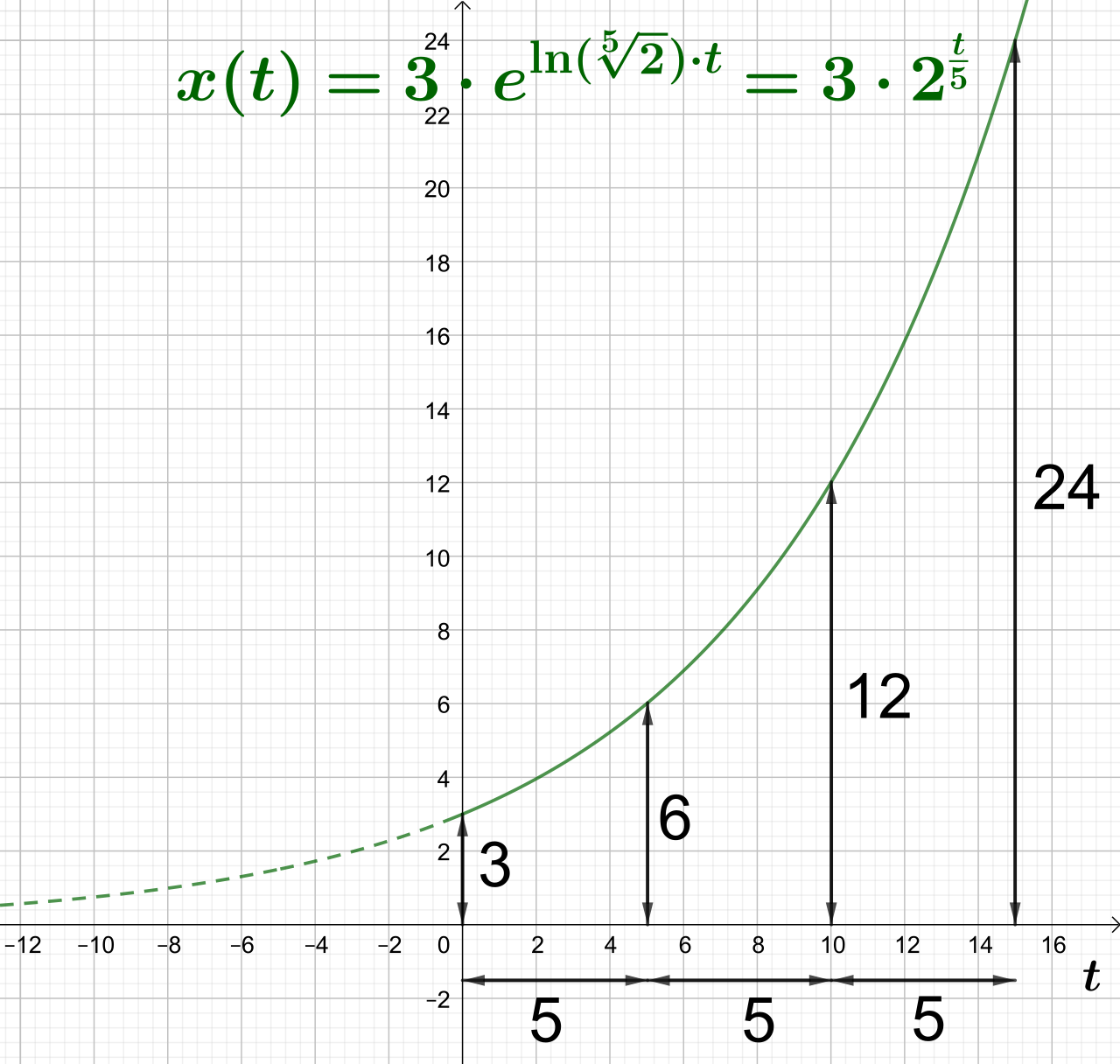
When plotted against their ordinal position numbers, the terms of a geometric sequence map along an exponential curve, with the common ratio acting as the base multiplier.

Just as the common difference mirrors linear slope, the common ratio has an algebraic counterpart. In a geometric sequence, the common ratio is equivalent to the base of an exponential function. If $y = a \cdot b^x$ , the base $b$ behaves exactly like the common ratio $r$ .

Real-world applications of geometric sequences are everywhere, driving the most powerful forces in economics and biology:

Real-world scenarios involving compound interest over discrete intervals can be modeled using geometric sequences. If an account earns $5\%$ compound interest, the balance is multiplied by $1.05$ each year.
Similarly, real-world scenarios involving population growth by a fixed percentage per discrete time period can be modeled using geometric sequences.

On the Praxis 5165 exam, you will frequently be required to translate fluently between these mathematical perspectives. The key to translating sequences is recognizing how the core parameters ( $d$ and $r$ ) manifest in each format.

Translating Arithmetic Formulas

When moving between forms, focus on the constant difference:

To translate a recursive arithmetic formula to an explicit formula, the added constant in the recursive step becomes the common difference in the explicit formula. If $a_n = a_{n-1} + 7$ , then $7$ takes the place of $d$ in $a_n = a_1 + (n-1)7$ .
To translate an explicit arithmetic formula to a recursive formula, the linear coefficient of $n$ becomes the common difference in the recursive step. Consider $a_n = 4n + 3$ . Because $4$ is the coefficient of $n$ (the "slope"), the common difference is $4$ . The recursive formula must be $a_n = a_{n-1} + 4$ .

Translating Geometric Formulas

When dealing with geometric patterns, track the multiplier:

To translate a recursive geometric formula to an explicit formula, the constant multiplier in the recursive step becomes the common ratio in the explicit formula. If $a_n = 3 \cdot a_{n-1}$ , then $3$ is the base in the explicit formula $a_n = a_1 \cdot 3^{n-1}$ .
To translate an explicit geometric formula to a recursive formula, the base of the exponent becomes the common ratio in the recursive step. In the explicit formula $a_n = 5 \cdot (0.8)^{n-1}$ , the base is $0.8$ . This means the sequence decays by multiplying by $0.8$ at each step, yielding the recursive step $a_n = 0.8 \cdot a_{n-1}$ .

Sequence Type	Core Feature	Recursive Form	Explicit Form	Translation Key
Arithmetic	Common Difference ( $d$ )	$a_n = a_{n-1} + d$	$a_n = a_1 + (n-1)d$	Added constant $\leftrightarrow$ Linear coefficient of $n$
Geometric	Common Ratio ( $r$ )	$a_n = r \cdot a_{n-1}$	$a_n = a_1 \cdot r^{n-1}$	Constant multiplier $\leftrightarrow$ Base of the exponent

As an educator, bridging the gap between abstraction and application often involves technology. Modern classrooms rely heavily heavily on graphing technology to visualize mathematics.

Graphing calculators evaluate recursive and explicit sequences using a specialized sequence graphing mode. When you switch a calculator like the TI-84 Plus from "Function" to "Seq" (Sequence) mode, the environment fundamentally changes. The standard $Y=$ screen is replaced by $u(n)$ , and the variable key inputs $n$ instead of $X$ .

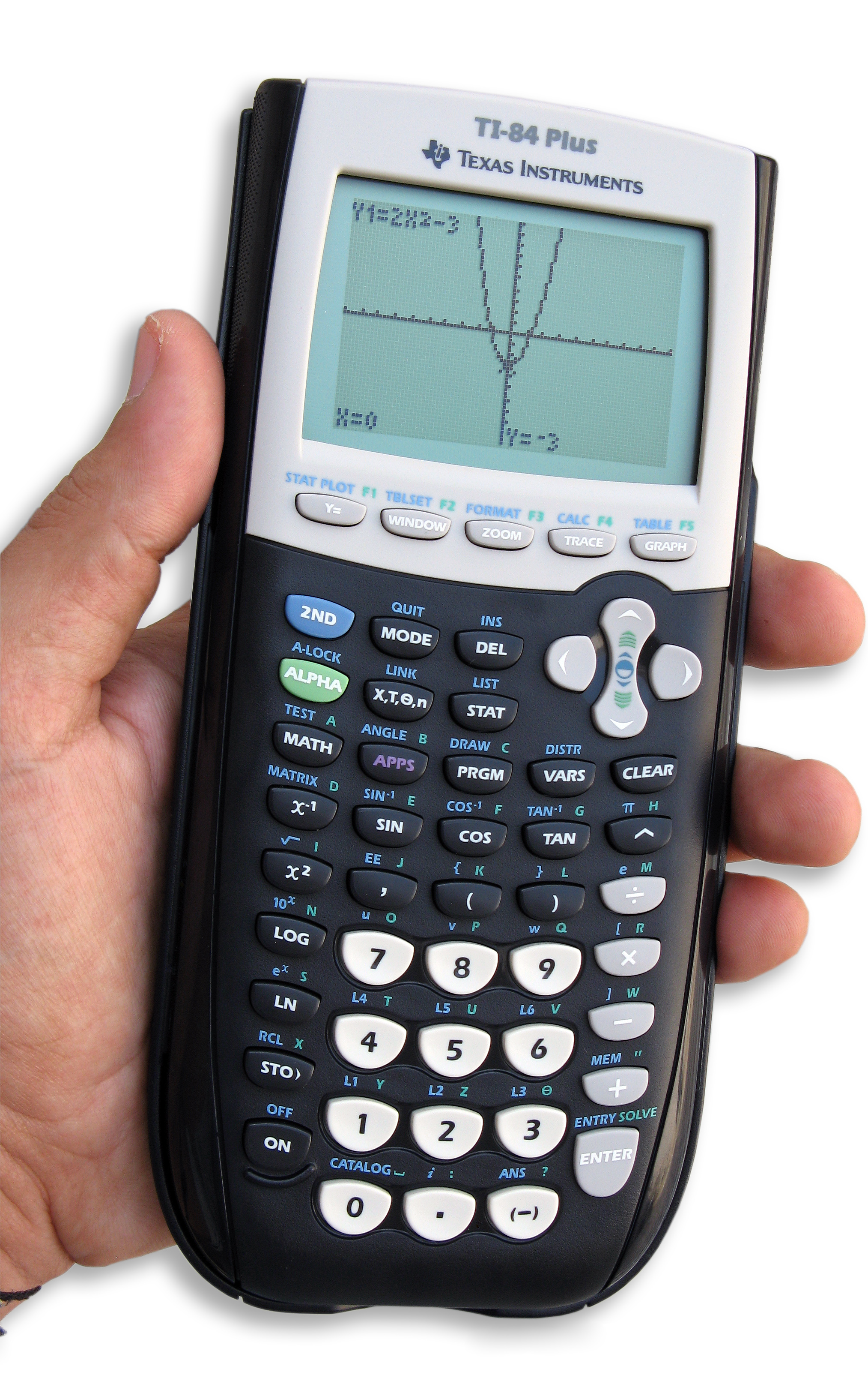
Graphing calculators feature a dedicated "Sequence" mode that enforces mathematical domain constraints by only accepting discrete integer inputs for position numbers.

Why is this pedagogical shift so crucial? Because it physically enforces the mathematical domain constraint. In function mode, a student can easily calculate $Y(2.5)$ . But in sequence mode, the calculator will only accept integer inputs for $n_{Min}$ , $n_{Max}$ , and the table parameters. By using sequence mode, you reinforce to the student that sequences are a progression of discrete events. You cannot evaluate a sequence at step $2.5$ any more than a bank can give you the $2.5$ th monthly interest payout.

Mastering these models—understanding their structure, graphing them accurately, and translating effortlessly between their explicit teleportation and recursive stepping-stones—equips you to help students model the precise, countable rhythms of the real world.