Linear, Quadratic, and Exponential Models
Not sure you’re ready?
Take the ~3-minute readiness diagnostic and see where you stand.
When your future students look at a data table, they are looking at the footprints of a function. The difference between adding three and multiplying by three seems trivial when examining the first few integers, but mathematically, it is the difference between a steady stroll and an explosive launch into the stratosphere. As a secondary mathematics teacher, your task is to teach students how to track these footprints—to distinguish the additive persistence of a linear model, the changing acceleration of a quadratic, and the relentless compounding of an exponential function.
Understanding these models is not merely an exercise in algebraic manipulation. It is about understanding how the universe grows, shrinks, and shifts. Whether your students are analyzing the decay of a carbon isotope, the trajectory of a thrown baseball, or the simple interest on their first savings account, they need a framework to map reality to mathematics.
To teach mathematical modeling effectively, we must first recognize the fundamental mechanic of change inherent in each function family. Data rarely arrives with a neat label; it is the pattern of growth that reveals the underlying model.
The Linear Walk
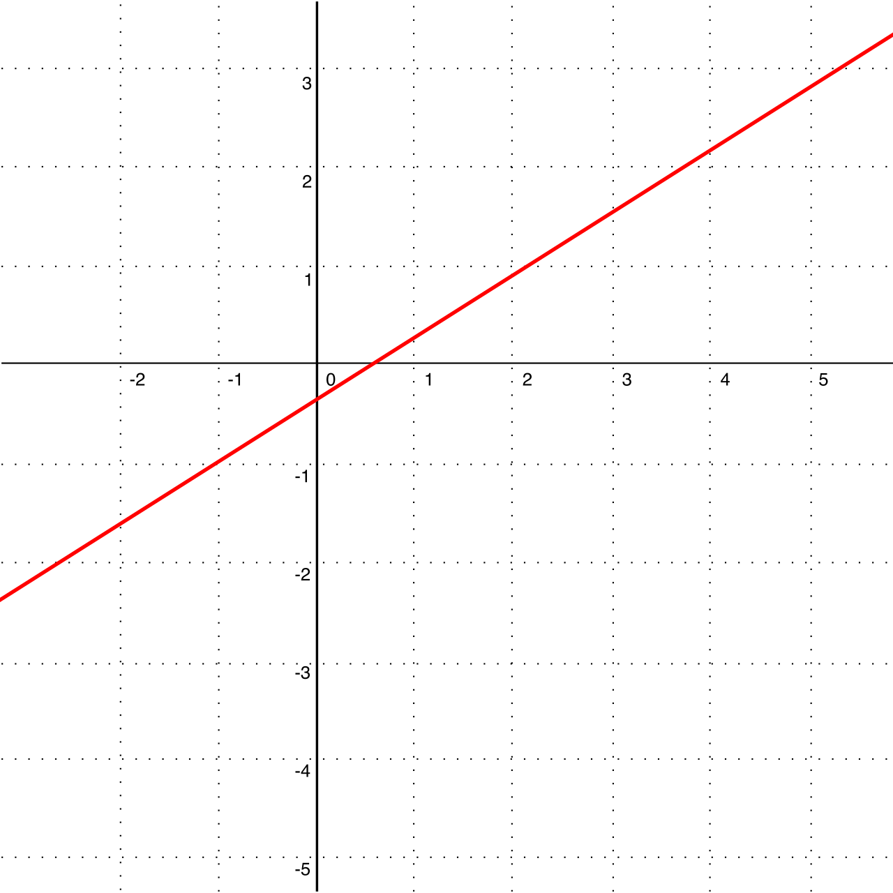
Linear functions change by a constant additive amount over equal intervals of the independent variable.
Think of a linear function as walking up a perfectly uniform staircase. For every step forward, you rise exactly the same amount. If we translate this to a tabular format, a linear function has a constant first difference between outputs for consecutive integer inputs. If f(1)=5, f(2)=8, and f(3)=11, the first difference is strictly +3.
Because of this strict additive nature, whenever you encounter a sequence with a constant difference between consecutive terms, it can be modeled by a discrete linear function. This is the foundation of arithmetic sequences.
The Quadratic Acceleration
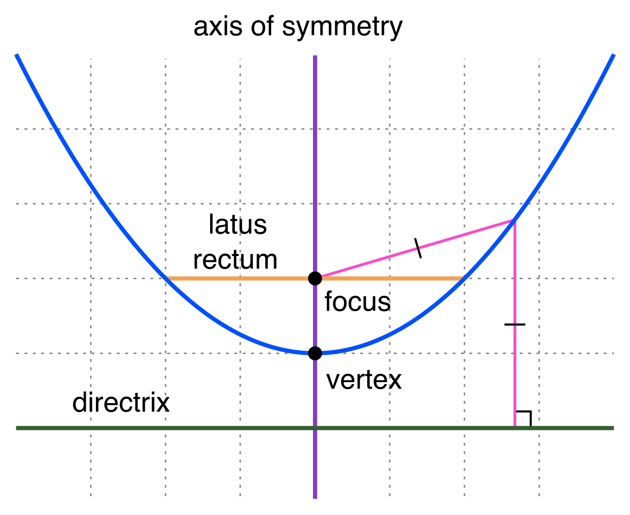
What happens if the steps themselves get larger at a steady rate? Here, we enter the quadratic domain. Quadratic functions have a constant second difference over equal intervals of the independent variable.
If you look at the sequence of perfect squares (1,4,9,16,25), the first differences are 3,5,7,9—these are clearly not constant. But if you take the differences of those differences (5−3, 7−5, 9−7), you get a constant +2. This constant second difference is the hallmark of quadratic growth. Visually, this changing rate of change causes the line to bend, meaning that the graph of a quadratic function is a parabola.
The Exponential Multiplier
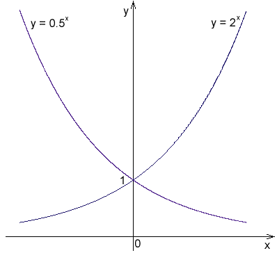
Now, imagine a scenario where growth is not based on adding, but on multiplying. Exponential functions change by a constant multiplicative factor over equal intervals of the independent variable.
Instead of adding $3 every day, what if a quantity triples every day? The sequence 2,6,18,54 yields wildly varying first and second differences. However, the ratio between terms (6/2, 18/6, 54/18) is always exactly 3. Thus, a sequence with a constant ratio between consecutive terms can be modeled by a discrete exponential function. This is the driving force behind geometric sequences.
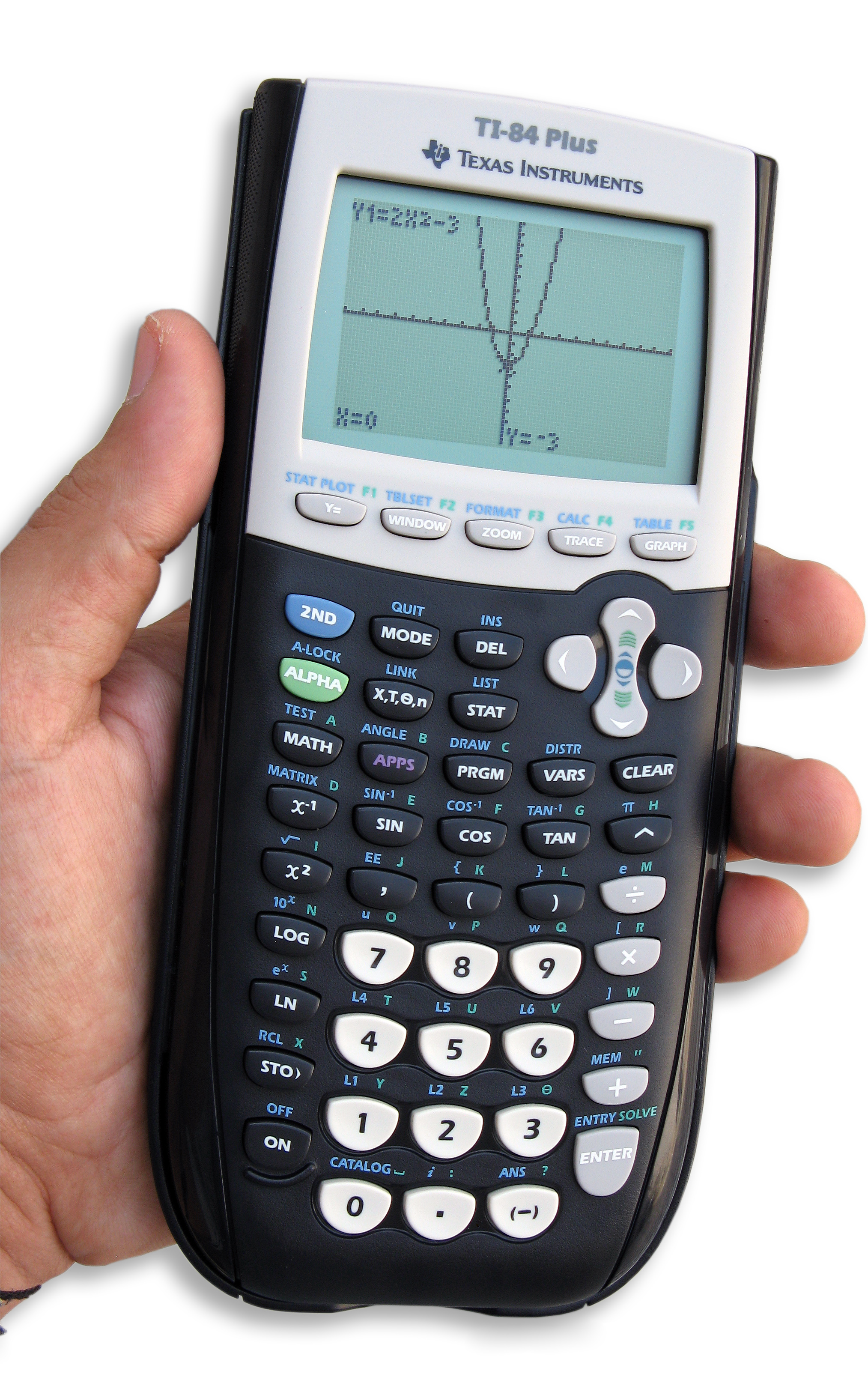
One of the most profound concepts you can explore with your students on a graphing calculator is the "race to infinity." If you set up a standard [−10,10] viewing window, a steep linear function might initially appear to outpace a gentle exponential curve. But mathematical truth reveals itself when we expand the domain.
- Linear vs. Quadratic: A steep line f(x)=100x looks dominant early on. However, a quadratic function with a positive leading coefficient will eventually produce larger values than any linear function for sufficiently large input values. The quadratic g(x)=0.1x2 may start slow, but around x=1000, the x2 term irrevocably crushes the linear term.
- Quadratic vs. Exponential: The parabola grows immensely fast, but it relies on an exponent that is fixed (x2). Exponential functions place the variable in the exponent (2x). Because of this, an exponential growth function will eventually produce larger values than any quadratic function for sufficiently large input values.
- Linear vs. Exponential: By logical extension, an exponential growth function will eventually produce larger values than any linear function for sufficiently large input values.
When your students trace y=1000x and y=1.01x on their calculators, they will see the line towering over the curve. But ask them to adjust their window's Xmax to 2000. Suddenly, the seemingly weak exponential function erupts upward, leaving the linear function in the dust.
When formulating models from word problems or datasets, you and your students must be fluent in the structural parameters of these functions. Let us deconstruct them.
Constructing Linear Functions
Standard Form: The standard slope-intercept form of a linear function is f(x)=mx+b.
In this model, the parameters have highly specific geometric and physical meanings:
- The variable m in the linear function f(x)=mx+b represents the constant rate of change.
- The variable b in the linear function f(x)=mx+b represents the initial value or y-intercept.
When bridging data to algebra, constructing a linear function from two points requires calculating the ratio of the difference in y-values to the difference in x-values to find the slope. Once m is known, b can be found by substituting a known point.
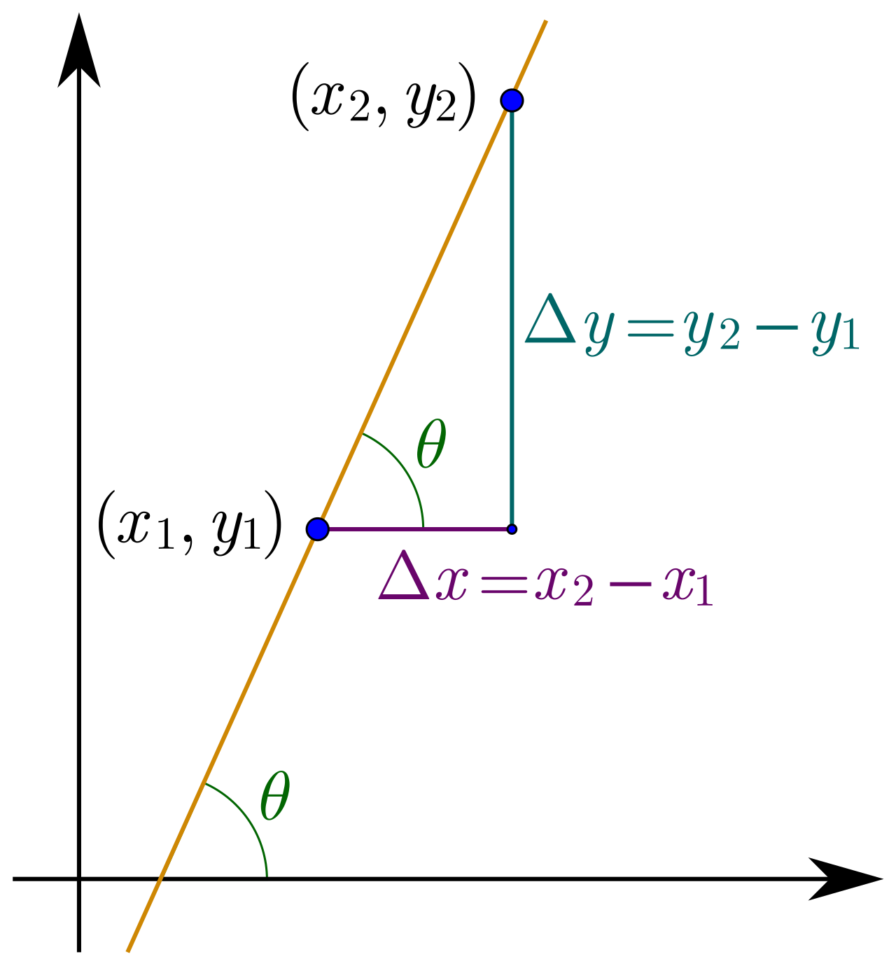
Real-world Context: If a student deposits $500 into an account that earns $25 a year, the account balance over time is f(x)=25x+500. Because the amount added is fixed, simple interest calculations represent linear growth over time.
Constructing Exponential Functions
Standard Form: The standard form of an exponential function is f(x)=a(b)x.
Exponential functions abandon additive slopes in favor of multipliers:
- The parameter a in the exponential function f(x)=a(b)x represents the initial value when x equals zero.
- The parameter b in the exponential function f(x)=a(b)x represents the constant growth or decay factor.
The behavior of the model hinges entirely on the value of b:
- An exponential function models growth when the base parameter is strictly greater than one. (e.g., b=1.05 represents a 5% increase).
- An exponential function models decay when the base parameter is strictly between zero and one. (e.g., b=0.85 represents a 15% decrease).
When looking at a graph of exponential decay (like a cooling cup of coffee), you will notice that the curve levels out but never truly reaches zero. Therefore, the graph of an exponential growth or decay function possesses a horizontal asymptote.
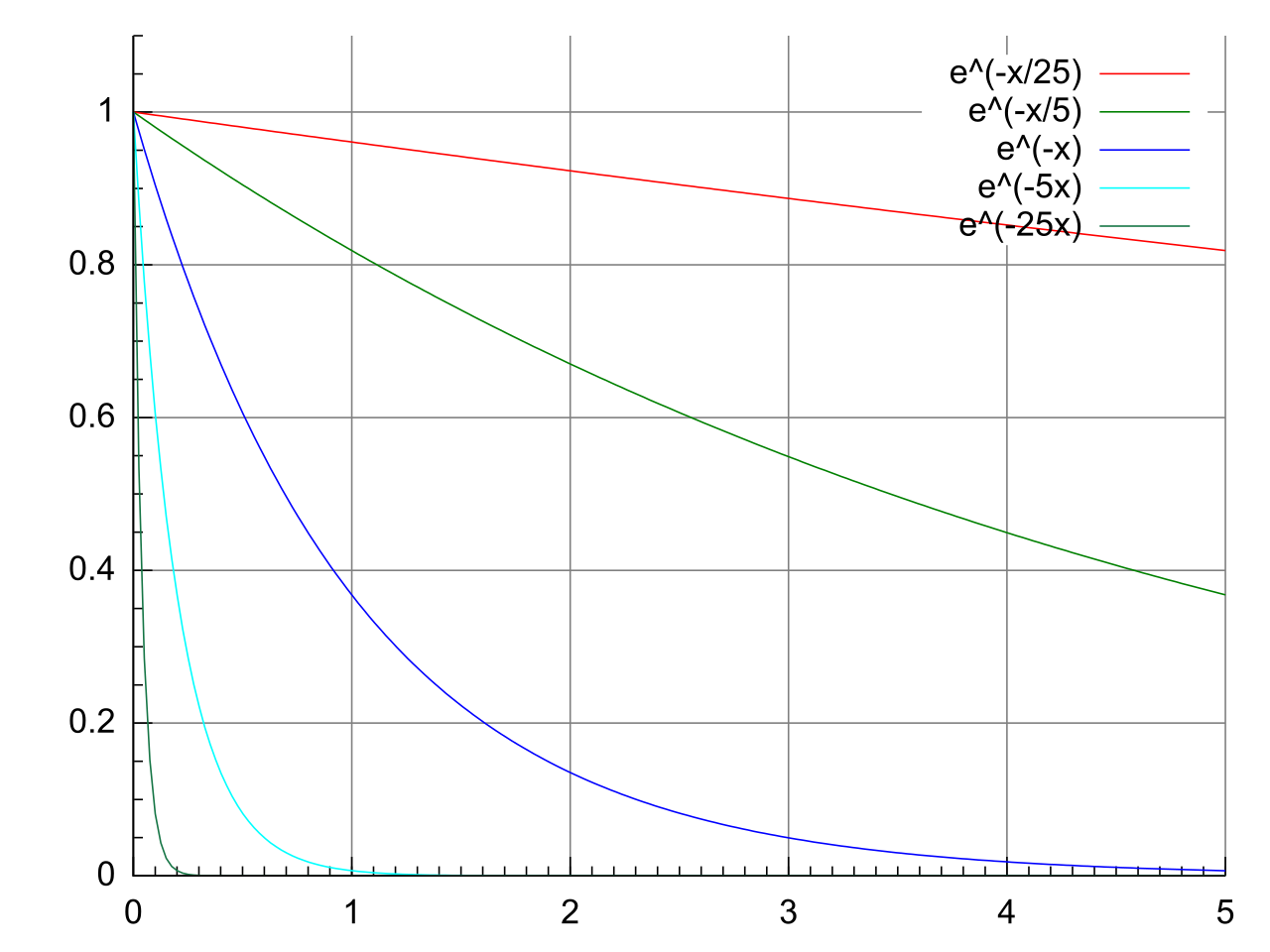
To extract this model from data: To find the base of an exponential function f(x)=a(b)x given two points with consecutive integer x-values, divide the y-value of the larger x by the y-value of the smaller x. (For instance, if f(3)=40 and f(4)=80, the base b=80/40=2).
Real-world Context: Unlike simple interest, compound interest calculations represent exponential growth over time. If interest is compounded continuously—meaning the compounding intervals are infinitely small—the standard base b transitions to a special mathematical constant. The continuous compound interest formula is A=Pert. In this beautiful formula, the mathematical constant e is approximately equal to 2.718. This constant acts as the universal speed limit for continuous compounding growth.
Calculus gives us the instantaneous rate of change (the derivative), but in Algebra 1 and 2, we rely heavily on the macroscopic view: the Average Rate of Change (AROC).
Definition: The average rate of change of a function f(x) over the interval from x=a to x=b is calculated as the quantity f(b) minus f(a) divided by the quantity b minus a. AROC=b−af(b)−f(a)
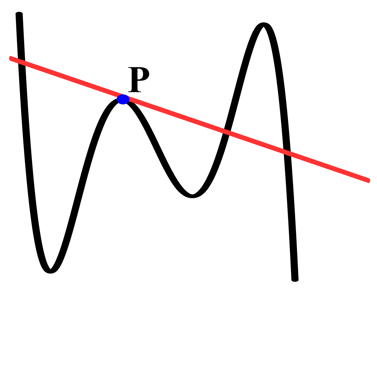
Geometrically, the average rate of change represents the slope of the secant line intersecting the graph of the function at x=a and x=b. Imagine a curvy, winding road representing a car's displacement over time. The secant line is the straight crow's-flight path from the start of the trip to the end. It ignores the slowing down and speeding up; it only cares about the net result.
Interpreting the AROC
The sign of the AROC tells a vital story about the interval:
- A positive average rate of change indicates that the function experiences an overall net increase over the given interval.
- A negative average rate of change indicates that the function experiences an overall net decrease over the given interval.
- An average rate of change of zero indicates no net change in the function value between the endpoints of the interval. (Note: This does not mean the function was flat the whole time; it merely means it finished exactly at the same height it started, like a thrown ball returning to the thrower's hand).
How AROC Behaves Across Function Families
The most profound distinction between our three function families can be observed by calculating their AROC over different, shifting intervals.
| Function Family | AROC Behavior | Conceptual Explanation |
|---|---|---|
| Linear | The average rate of change of a linear function remains constant regardless of the specific interval chosen. | Because a line has a uniform slope, any secant line you draw on it will perfectly overlay the line itself. The AROC is always exactly m. |
| Quadratic | The average rate of change of a quadratic function varies depending on the specific interval chosen. | On a parabola, secant lines get progressively steeper as you move away from the vertex. The rate at which the AROC changes is, itself, constant (linking back to the constant second difference). |
| Exponential | The average rate of change of an exponential function varies depending on the specific interval chosen. | As the curve bends exponentially upward (or downward), the secant lines become radically steeper. The AROC of an exponential function actually grows exponentially! |
Pedagogical Takeaway
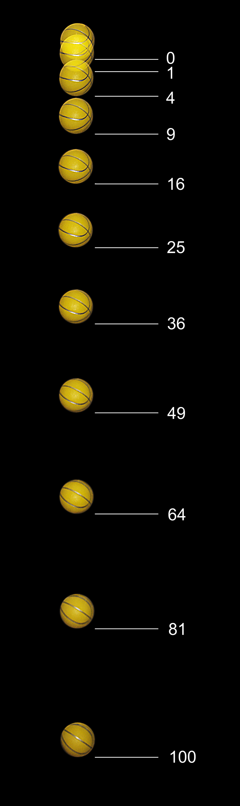
When you prepare your students for high-stakes assessments, emphasize why these models exist. A linear model is an agreement of total fairness—every interval gets the exact same amount. A quadratic model is an agreement of steady acceleration—gravity pulling a falling object faster and faster. An exponential model is a snowball rolling down a hill—where the current size of the snowball dictates how much more snow it can gather.
Mastering these core principles will not only allow you to breeze through the constructed-response and selected-response items on your Math 5165 exam; it will give you the precise, vivid language required to make these concepts sing in your future classroom.