Expected Values and Decisions

To perform mathematics on chance, we must first capture it. We do this through the concept of a random variable, which is simply a variable whose possible values are numerical outcomes of a random phenomenon. Think of a random variable as a function that assigns a number to every possible outcome of an unpredictable event.

Source: Random Variable as a Function-en by Niyumard, CC BY-SA 4.0.

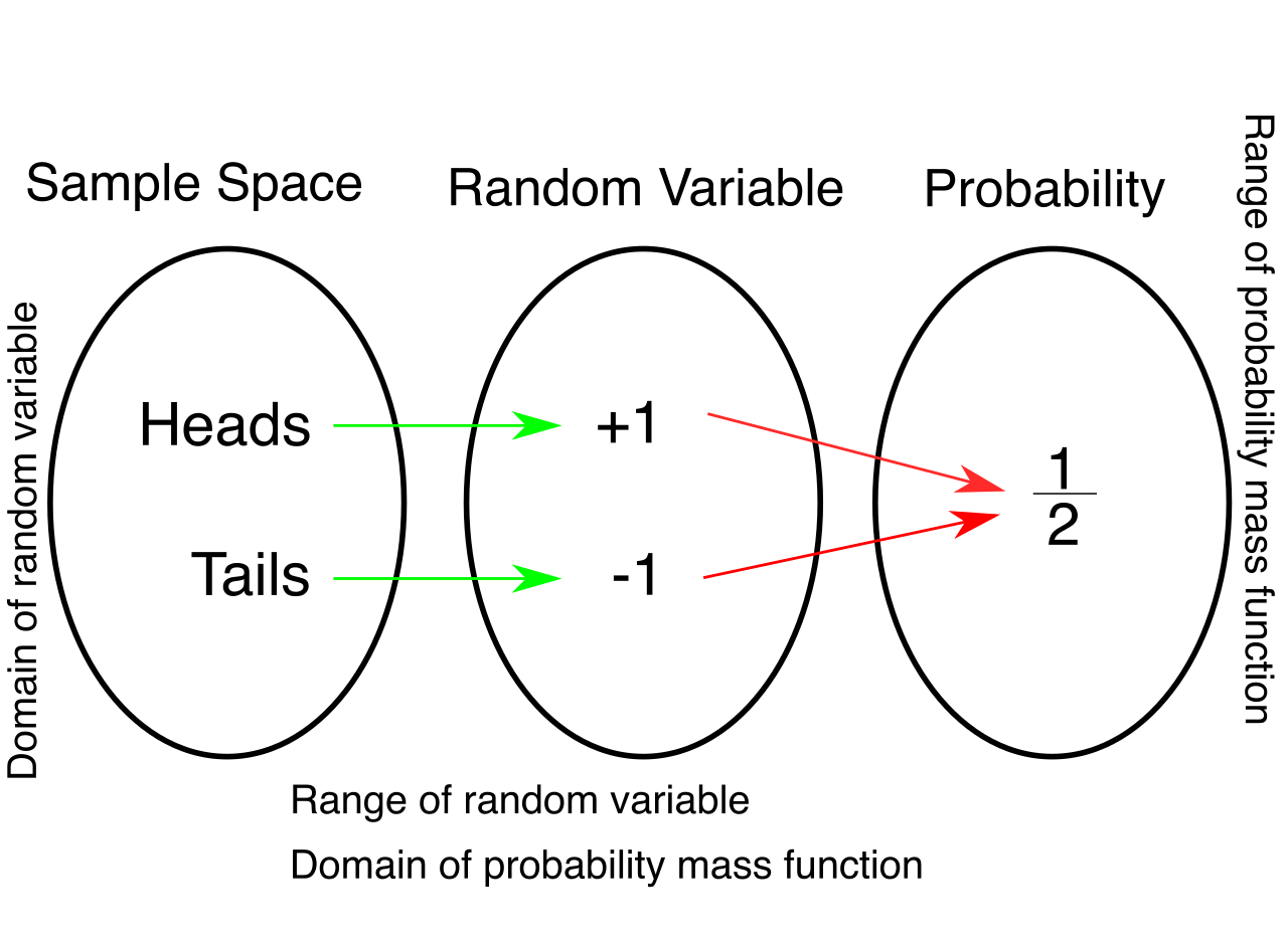
Depending on the nature of the data, random variables take one of two forms:

• A discrete random variable has a countable number of possible values. The number of correct answers a student guesses on a ten-question quiz, the number of defects in a batch of graphing calculators, or the face showing on a rolled die are all discrete. You can count them: 0, 1, 2, 3...
• Conversely, a continuous random variable takes all values in an interval of numbers. The exact time it takes a student to complete an exam, or the precise distance a javelin is thrown, are continuous. There is an infinite, uncountable continuum of possible measurements.

For decisions involving discrete scenarios—like games of chance or standardized test scoring—we rely on the discrete random variable.

To understand a discrete random variable, we must know not just what values it can take, but how often it takes them. A probability distribution of a discrete random variable provides the probability of each possible value.

Building a valid probability distribution requires strict architectural rules. Expected value calculations require mutually exclusive and exhaustive outcomes to accurately represent a complete decision scenario. "Mutually exclusive" means no two outcomes can happen simultaneously; "exhaustive" means every possible outcome is accounted for.

Because of this requirement, two ironclad axioms govern the distribution:

1. Bounded Probabilities: Every probability assigned to a specific value in a discrete probability distribution must be a number between zero and one, inclusive ($0 \le P(x) \le 1$). A probability cannot be negative, nor can it exceed 100%.
2. The Rule of Total Probability: The sum of the probabilities of all possible values in a discrete probability distribution must exactly equal one ($\sum P(x) = 1$). You have accounted for 100% of the universe of possibilities.

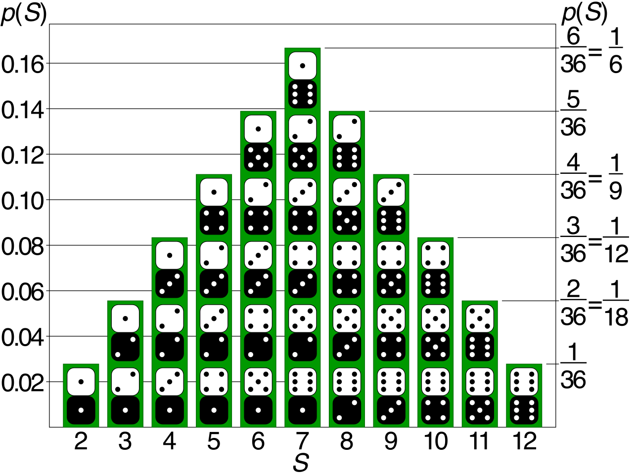
We can illustrate this beautifully. A probability histogram visually represents a discrete probability distribution with the total area of all bars summing exactly to one. The x-axis denotes the possible numerical outcomes, and the y-axis denotes their probabilities. Because the width of each bar is typically 1 unit, the area of each bar is equal to its probability, making the geometry of the histogram perfectly match the algebra of the distribution.

Nature is noisy in the short term, but exceptionally orderly in the long term. This order is captured by the expected value. The expected value of a discrete random variable is the long-run average outcome of a random process repeated infinitely many times.

If your students flip a coin and win $2 for heads and lose $1 for tails, the outcome of a single flip is pure chance. But over thousands of flips, a predictable average emerges.

Calculating Expected Value The expected value of a discrete random variable is calculated by multiplying each possible value by its probability and adding these products together.

$E(X) = \sum [x \cdot P(x)]$

The symbol used to represent the expected value of a random variable $X$ is $E(X)$. In terms of its theoretical foundation, the expected value of a random variable is mathematically equivalent to the mean of the random variable. Because of this equivalence, the Greek letter $\mu$ (mu) is conventionally used to denote the expected value or mean of a probability distribution.

Source: Beta first moment by Erzbischof, CC BY-SA 3.0.

The Paradox of the "Expected" Outcome

A common cognitive hurdle for students is the word "expected." An expected value of a random variable is not required to be an actual possible outcome of the random variable.

Consider a standard six-sided die. The possible values are 1, 2, 3, 4, 5, and 6, each with a probability of $\frac{1}{6}$. $E(X) = 1(\frac{1}{6}) + 2(\frac{1}{6}) + 3(\frac{1}{6}) + 4(\frac{1}{6}) + 5(\frac{1}{6}) + 6(\frac{1}{6}) = 3.5$

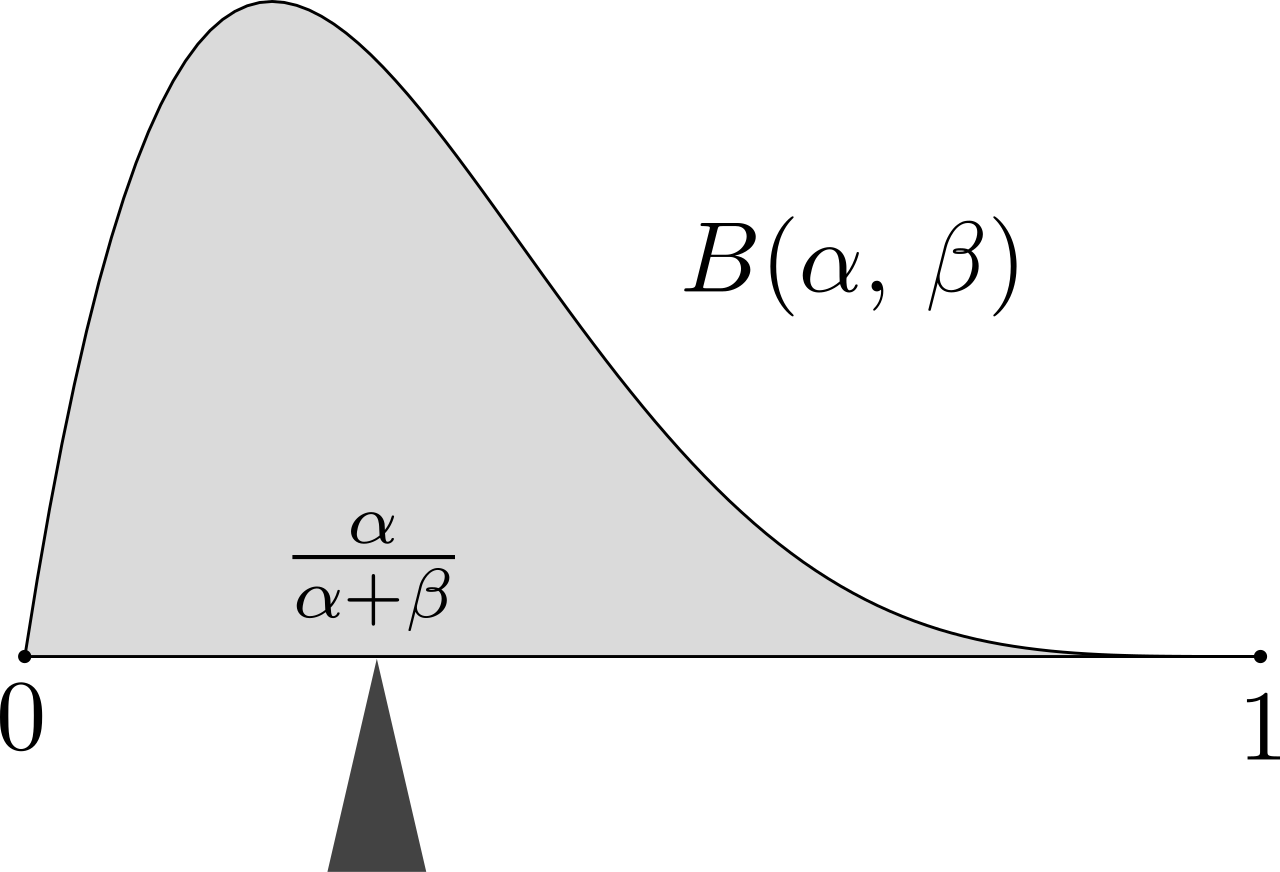
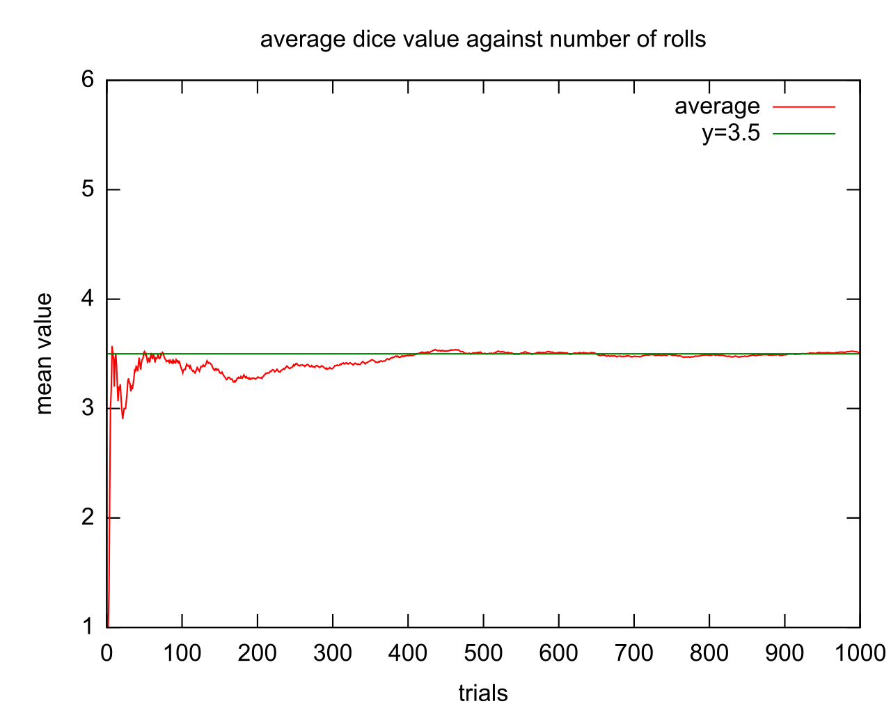
The expected value is 3.5. You will never, ever roll a 3.5. Yet, 3.5 perfectly describes the center of gravity of the distribution. Why does this matter? Because the Law of Large Numbers dictates that the empirical average of independent trials approaches the expected value as the number of trials increases. If you roll that die ten thousand times and average the results, your calculator will show a number incredibly close to 3.5.

Expected values behave with elegant algebraic predictability, which makes them powerful tools for manipulating grading scales or financial models.

1. Linearity (Scaling and Shifting) For any random variable $X$ and constants $a$ and $b$, the expected value of $aX$ plus $b$ equals $a$ times the expected value of $X$, plus $b$: $E(aX + b) = aE(X) + b$

Teaching Context: Imagine your class takes a notoriously difficult exam. The expected score is $\mu = 40$. You decide to curve the exam by doubling everyone's score ($a = 2$) and adding 5 bonus points ($b = 5$). What is the new expected average? You do not need to recalculate every student's probability. The new expected value is simply $2(40) + 5 = 85$.

2. Additivity of Random Variables For any two random variables $X$ and $Y$, the expected value of $X$ plus $Y$ equals the expected value of $X$ plus the expected value of $Y$: $E(X + Y) = E(X) + E(Y)$

Teaching Context: If a student enters a school carnival and plays the Ring Toss (where the expected prize value is $1.50) and the Dunk Tank (where the expected prize value is $2.00), the expected total prize value they walk away with is simply $3.50. Remarkably, this property holds true even if the random variables are dependent.

Once we can calculate the expected value, we can use it to engineer rational decisions. When faced with multiple choices, we construct a decision matrix, which uses expected values to compare the average long-term payoffs of different available actions under uncertainty.

Games of Chance and Fairness

In game theory and probability curricula, we frequently analyze whether a game is "fair." In the vernacular, "fair" means rules are applied equally. In mathematics, a mathematically fair game is a game in which the expected net winnings for a player equal exactly zero. Over the long run, neither the player nor the house gains or loses money.

To evaluate this in the real world, we must account for the buy-in. If a game costs money to play, the expected net profit is calculated as the expected gross payout minus the initial cost of playing.

Let us design a carnival game:

• Cost to play: $5
• Payout: You roll a die. If you roll a 6, you win $12. Otherwise, you win nothing.

First, find the expected gross payout: E(\text{Gross}) = \12(\frac{1}{6}) + $0(\frac{5}{6}) = $2.00$

Now, find the expected net profit: E(\text{Net}) = E(\text{Gross}) - \text{Cost} = \2.00 - $5.00 = -$3.00$

For every time a student plays this game, they should expect to lose $3.00 on average. Because the expected net winnings do not equal zero, this is not a mathematically fair game. (It is, however, an excellent fundraiser for the math club).

Risk and Real-World Applications

This exact calculus is the bedrock of the global financial system. Insurance companies determine base policy premiums by calculating the expected value of the policy payout for a given risk class.

If an auto insurer knows that a specific demographic of drivers has a 1% chance of causing $50,000 in damages and a 99% chance of causing $0 in damages in a given year, the expected payout is: E(\text{Payout}) = \50,000(0.01) + $0(0.99) = $500$

The insurer's expected cost is $500 per driver. To stay in business, they will set the base premium slightly above $500. Over millions of drivers (invoking the Law of Large Numbers), the insurer's actual average payout will converge almost exactly to the expected value, guaranteeing profitability.

When an institution operates this way, they are practicing risk-neutral decision making, which involves consistently choosing the option with the highest expected value regardless of outcome variance. An insurance company does not fear the variance of a single $50,000 payout because they are playing the infinite game. They trust the expected value. As mathematics educators, our objective is to teach students how to uncover this hidden order, empowering them to weigh their own choices against the inescapable laws of probability.