Probability Rules and Counting

Not sure you’re ready?

Take the ~3-minute readiness diagnostic and see where you stand.

To study probability is to map the architecture of the possible. As future secondary mathematics educators, you will frequently encounter students who view probability and combinatorics as a dizzying grab-bag of disconnected formulas—a chaotic lottery of factorials and fractions. Your task, and the focus of the Praxis (5165): Mathematics exam, is to demystify this space. You must reveal that counting and probability are entirely deterministic disciplines of logic. We are simply keeping an exact, rigorous ledger of universes that could exist. Whether a student is trying to crack a password, draw a flush, or determine the likelihood of an entirely unpredictable sequence of events, they are fundamentally engaged in the mathematics of sets and systematic counting. Let us build the canonical framework you will use to guide them.

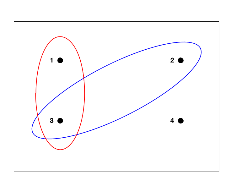
Before we can calculate the likelihood of an event, we must define the universe in which it lives. A sample space is defined as the set of all possible outcomes of a probabilistic experiment. It is the boundary of our mathematical reality for any given problem.

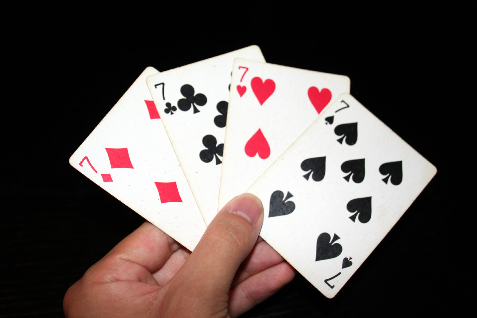
A visual representation of a finite sample space, demonstrating how distinct events are bounded within the universal set of possible outcomes.

When you roll a standard six-sided die, you are operating within a sample space of faces numbered with the integers 1 through 6. When you draw from a standard deck of playing cards, your sample space contains exactly 52 cards. This deck is divided into exactly four suits—hearts, diamonds, clubs, and spades—and each suit contains exactly 13 cards.

The four standard playing card suits: diamonds, clubs, hearts, and spades. Each suit contains 13 cards, creating a uniform sample space of 52 distinct outcomes.

If every outcome in our sample space is equally likely, we are operating in a uniform sample space. Here, the theoretical probability of an event is simply the number of favorable outcomes divided by the total number of possible outcomes.

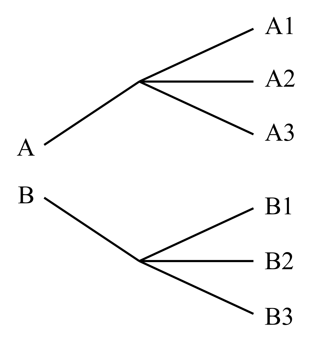
But how do we count those outcomes when the sample space grows overwhelmingly large? We rely on the fundamental counting principle, which states that the total number of outcomes for a sequence of events is the product of the number of outcomes for each individual event. Consequently, the probability of a sequence of independent trials is calculated by multiplying the individual probabilities of each trial.

A visual demonstration of the fundamental counting principle, showing how the elements of two distinct sets combine to create a total number of compound outcomes equal to their product.

When a student attempts to guess a forgotten password or assign unique characters to a license plate, the sequence of the characters is paramount. Problem scenarios involving passwords or license plates typically require permutation formulas because the sequence of characters matters.

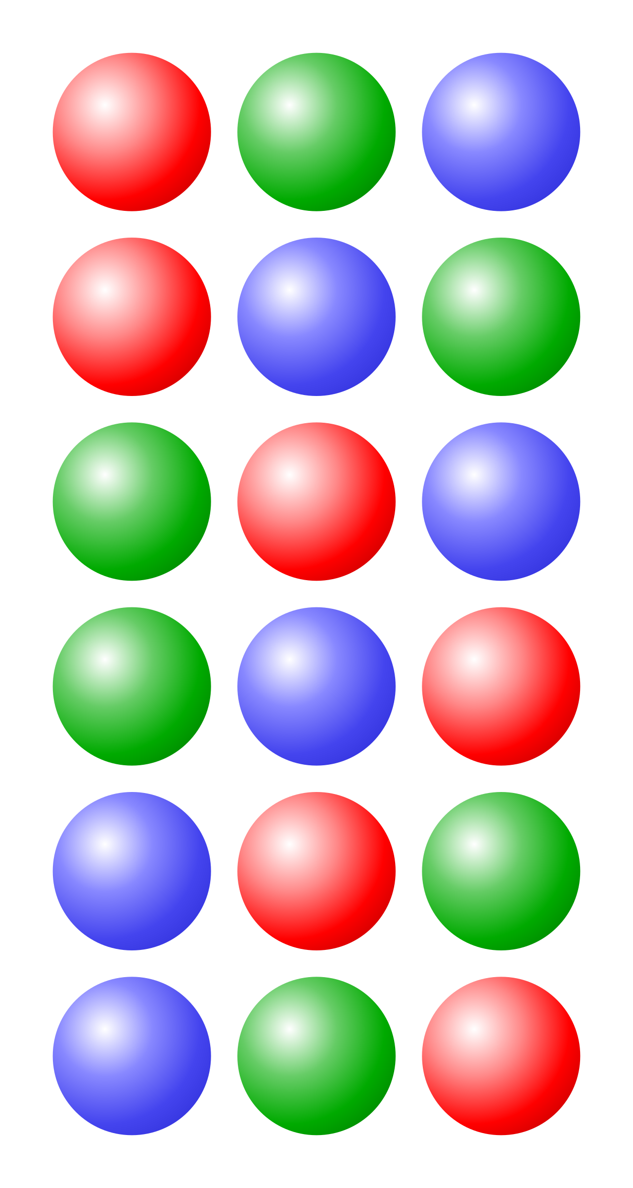
A permutation is an arrangement of objects in a specific sequence. In a permutation of a set of objects, the order of the objects is critical to the arrangement. To calculate these arrangements, we use the mathematical operation called a factorial, represented by the symbol !. The factorial of a positive integer $n$ is the product of all positive integers less than or equal to $n$ .

Crucial Boundary Values:

The numerical value of one factorial ($1!$) is exactly 1.

The numerical value of zero factorial ($0!$) is exactly 1. (There is exactly one way to arrange zero objects: do nothing).

Permuting Distinct Objects

The formula for the number of permutations of $n$ distinct objects taken $r$ at a time is:

$_nP_r = \frac{n!}{(n - r)!}$

If you want to arrange all your objects, the math simplifies elegantly. The number of permutations of $n$ distinct objects arranged in a single line is $n!$ . Therefore, the value of $_nP_n$ , representing permuting all $n$ items from $n$ items, is equal to $n!$ . Conversely, the value of $_nP_0$ , representing permuting 0 items from $n$ items, is always 1.

The six unique permutations of three distinct objects. Because the sequence matters, rearranging the same three items creates a mathematically distinct outcome.

Variations on Permutations

The real world is rarely composed of purely distinct, linearly arranged objects. You must be prepared to teach two crucial variations:

Indistinguishable Objects: What if you are rearranging the letters in the word "MISSISSIPPI"? The formula for the number of distinguishable permutations of $n$ objects where some objects are identical is:

$\frac{n!}{n_1! \times n_2! \times \dots \times n_k!}$ In the distinguishable permutations formula, the values $n_1, n_2, \dots, n_k$ represent the frequencies of each distinct type of identical object within the total $n$ objects.
Circular Arrangements: If you seat people around a circular dinner table, there is no "first" or "last" seat. Because shifting everyone one seat to the left results in the exact same relative seating arrangement, circular permutations of $n$ distinct objects can be arranged in exactly $(n - 1)!$ distinct ways.

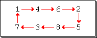
In a cyclic permutation, shifting the sequence by one position results in the same relative arrangement, illustrating why the formula (n-1)! is necessary to eliminate duplicate circular orderings.

Often, we only care about who is in the room, not the order in which they walked through the door. Problem scenarios involving committee formations or handshakes typically require combination formulas because the sequence of selection does not matter.

A combination is a selection of objects from a larger group where the order of selection is irrelevant. The formula for the number of combinations of $n$ distinct objects taken $r$ at a time is:

$_nC_r = \frac{n!}{r!(n - r)!}$

Choosing exactly 3 elements from a set of 5 distinct items yields 10 possible combinations. Unlike permutations, the internal order of the selected items does not matter.

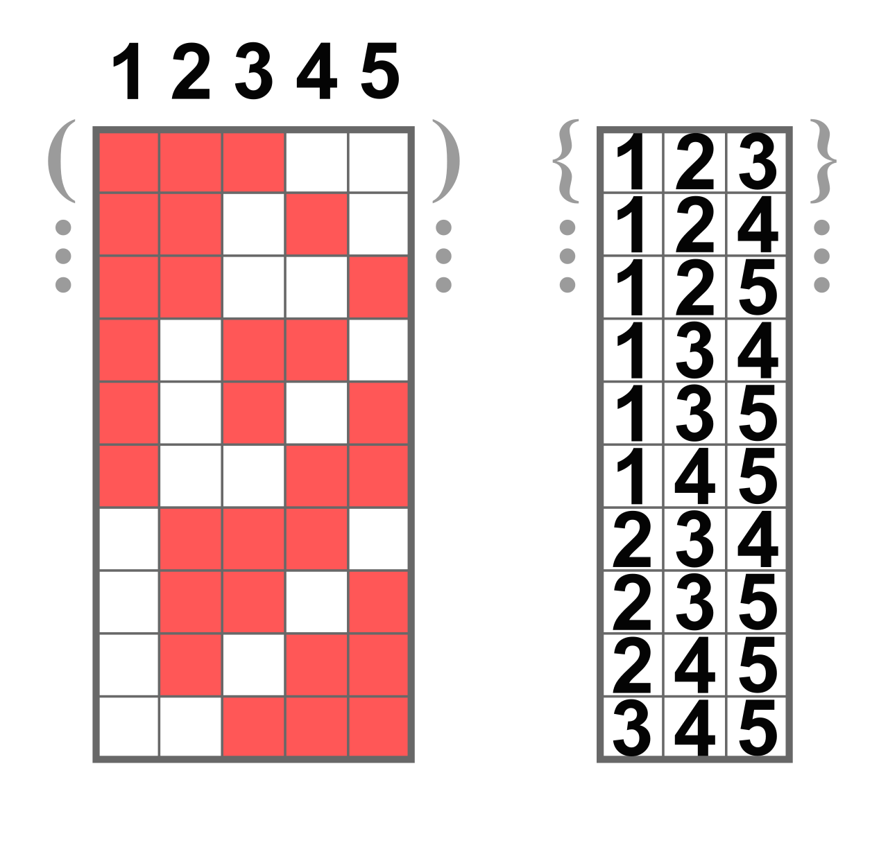
The value of the combination $_nC_r$ is mathematically equivalent to the binomial coefficient ' $n$ choose $r$ '.

Combinations possess a beautiful, intuitive symmetry. Every time you choose $r$ objects to keep, you are simultaneously choosing $n-r$ objects to leave behind. Thus, the mathematical identity $_nC_r = \_{n}C_{n-r}$ reflects the symmetry of combinations. Furthermore, the value of $_nC_0$ , representing choosing 0 items from $n$ items, is always 1. Symmetrically, the value of $_nC_n$ , representing choosing all $n$ items from $n$ items, is always 1.

When calculating likelihoods in these scenarios, the probability of selecting a specific combination of items is simply the number of favorable combinations divided by the total number of possible combinations.

The Stars and Bars Method

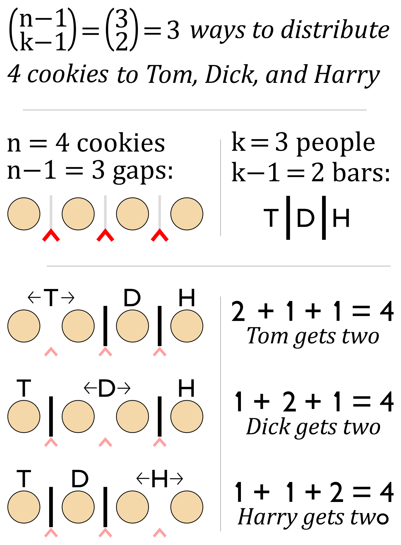
What happens when you need to distribute identical objects into distinct categories? Suppose you have $n$ identical pieces of candy to distribute among $k$ different students. Because the candy is identical, combinations of distinct objects fail us.

Here, we use a brilliant technique called the stars and bars method. It is used to find the number of ways to distribute identical items into distinct bins. Imagine the $n$ items as stars ( $\star$ ), and place $k-1$ bars ( $|$ ) among them to divide the stars into $k$ distinct bins. The formula for the number of ways to distribute $n$ identical items into $k$ distinct bins is:

$_{n + k - 1}C_{k - 1}$

The stars and bars method uses dividers to partition identical objects into distinct groups, transforming an indistinguishable distribution problem into a calculable combination.

In the classroom, you will frequently transition from counting outcomes to evaluating consecutive events. The mechanics of these calculations hinge entirely on whether one event remembers the other.

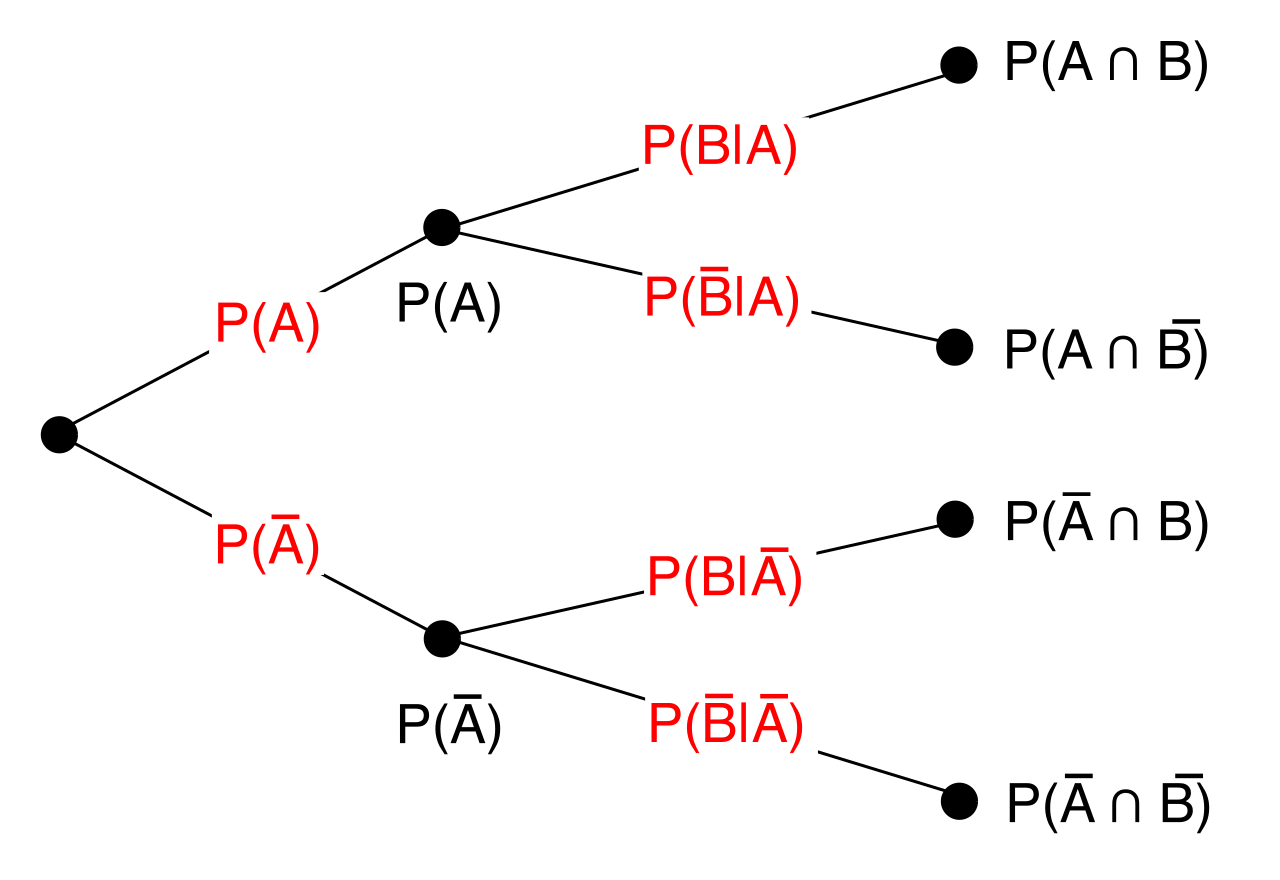
The general multiplication rule formula is:

$P(A \text{ and } B) = P(A) \times P(B|A)$

The notation $P(B|A)$ represents the conditional probability of event $B$ occurring given that event $A$ has already occurred.

Tree diagrams effectively map the general multiplication rule, illustrating how the probability of secondary branches is conditional on the specific outcome of the preceding event.

Dependent vs. Independent Sampling

Sampling objects without replacement means that each selection forms a dependent event. If you draw an Ace from a standard deck and do not replace it, the deck has fundamentally changed. The conditional probability $P(B|A)$ will differ from the original probability $P(B)$ .
Sampling objects with replacement means that each selection forms an independent event. The deck is reset.

Two events are independent if the occurrence of one event does not affect the probability of the other event. Mathematically, for independent events $A$ and $B$ , the conditional probability $P(B|A)$ is equal to the marginal probability $P(B)$ . Because of this equality, the formula for the multiplication rule applied to independent events simplifies beautifully:

$P(A \text{ and } B) = P(A) \times P(B)$

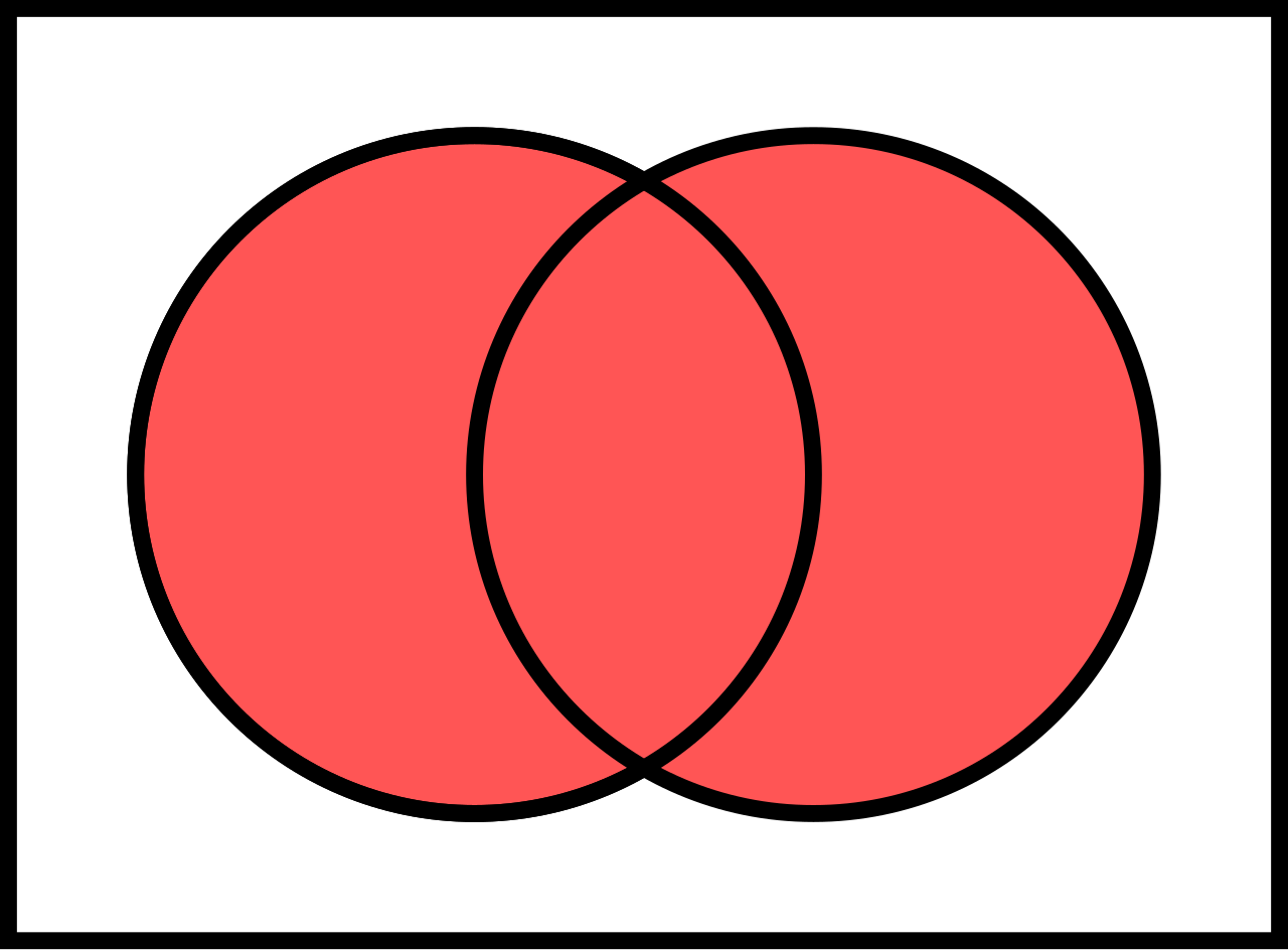
When a student asks, "What is the probability of drawing a Heart or a Face card?", they are asking for the union of two sets.

The general addition rule formula is:

$P(A \text{ or } B) = P(A) + P(B) - P(A \text{ and } B)$ We subtract the intersection $P(A \text{ and } B)$ to correct for double-counting the outcomes where both events overlap (the King, Queen, and Jack of Hearts).

However, what if we ask for the probability of drawing a Heart or a Spade? These are mutually exclusive events, which are defined as events that cannot occur at the same time. For mutually exclusive events $A$ and $B$ , the probability of the intersection of event $A$ and event $B$ is exactly zero. Because $P(A \text{ and } B) = 0$ , the addition rule formula for mutually exclusive events simplifies to:

$P(A \text{ or } B) = P(A) + P(B)$

A Venn diagram depicting the union of two sets. When events overlap, their intersection must be subtracted to avoid double-counting. If events are mutually exclusive, they share no overlapping space.

The Principle of Inclusion-Exclusion for Three Events

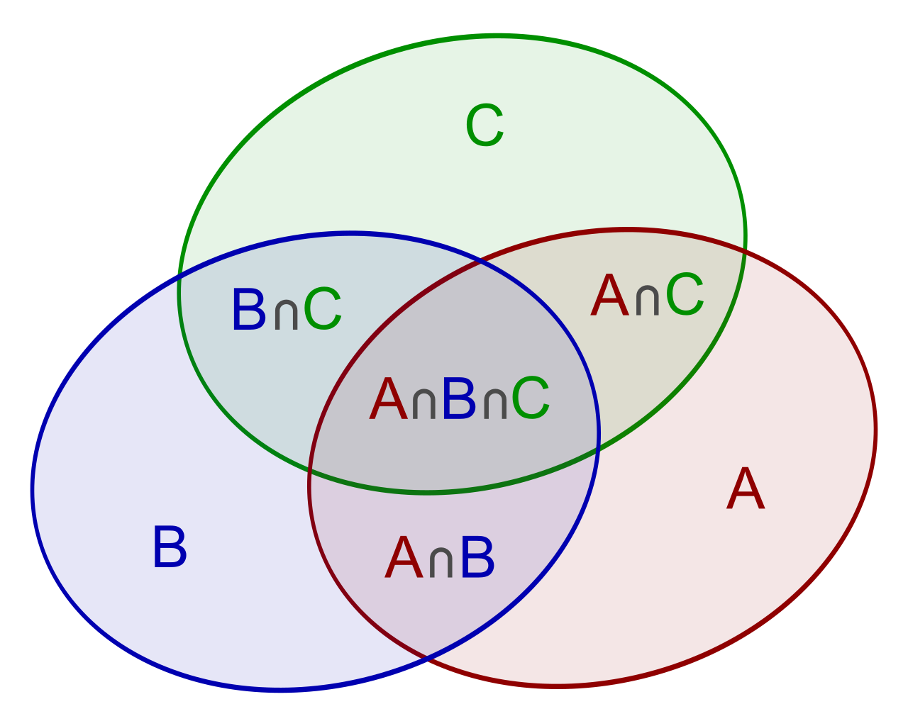
As systems grow more complex, you must track overlaps meticulously. If a student analyzes three intersecting sets (A, B, and C), they must apply the Principle of Inclusion-Exclusion:

$P(A \text{ or } B \text{ or } C) = P(A) + P(B) + P(C) - P(A \text{ and } B) - P(A \text{ and } C) - P(B \text{ and } C) + P(A \text{ and } B \text{ and } C)$

Why do we add the final term? When we subtract all the two-way intersections, we inadvertently subtract the exact center (where all three overlap) one time too many. We must add it back to balance our universal ledger.

The Principle of Inclusion-Exclusion applied to three intersecting sets. To find the total union without double-counting, you add the individual areas, subtract the two-way overlaps, and add back the central three-way intersection.

Sometimes, counting the ways an event can happen is agonizingly complex, while counting the ways it cannot happen is trivial.

The complement of event $A$ consists of all outcomes in the sample space that are not included in event $A$ . The notation $P(A')$ represents the probability of the complement of event $A$ . Because the sample space is the sum total of all possibilities, the sum of the probability of an event and the probability of the complement of that same event always equals 1.

This gives us the fundamental formula relating the probability of an event $A$ and the probability of the complement of event $A$ :

$P(A') = 1 - P(A)$

For exam candidates and future teachers alike, this unlocks one of the most powerful shortcuts in probability: the "at least one" trick. Imagine rolling ten dice and calculating the probability of getting at least one six. Calculating exactly one, exactly two, exactly three... all the way to ten is mathematically exhausting.

Instead, we shift our perspective to the complement. Calculating the probability of 'at least one' success is equivalent to subtracting the probability of 'zero successes' from 1.

$P(\text{at least one}) = 1 - P(\text{none})$

By mastering this perspective shift, you equip yourself not just to pass the Praxis 5165, but to show your future students the profound elegance of mathematical modeling. The rules of probability are not arbitrary hoops to jump through; they are the precise, logical translations of common sense into the language of mathematics.