Linear Regression and Correlation

Not sure you’re ready?

Take the ~3-minute readiness diagnostic and see where you stand.

Imagine dropping a scatter of pushpins onto a map to mark the locations of high schools and their average standardized test scores. The eye naturally wants to draw a line through the chaos, searching for a rhythm in the noise. This innate human desire to find patterns is formalized in the mathematics of linear regression. As future educators, you will look at data every day—from tracking attendance versus academic performance to measuring the hours students spend on homework against their unit exam grades. Understanding how to rigorously model these relationships, while knowing exactly where these models break down, separates the passive consumer of data from the precise architect of instruction.

In this text, we will unpack the mechanics of linear regression and correlation, building the intuition required not just to pass your licensure exam, but to confidently teach these concepts to your future students.

When we analyze bivariate data, we are often asking a simple question: If I know something about one trait, what does that tell me about another?

A linear regression function models the linear relationship between an explanatory variable (the input, typically plotted on the x-axis) and a response variable (the output, plotted on the y-axis). When we create this model, we are constructing a hypothetical line that best captures the trend of the data.

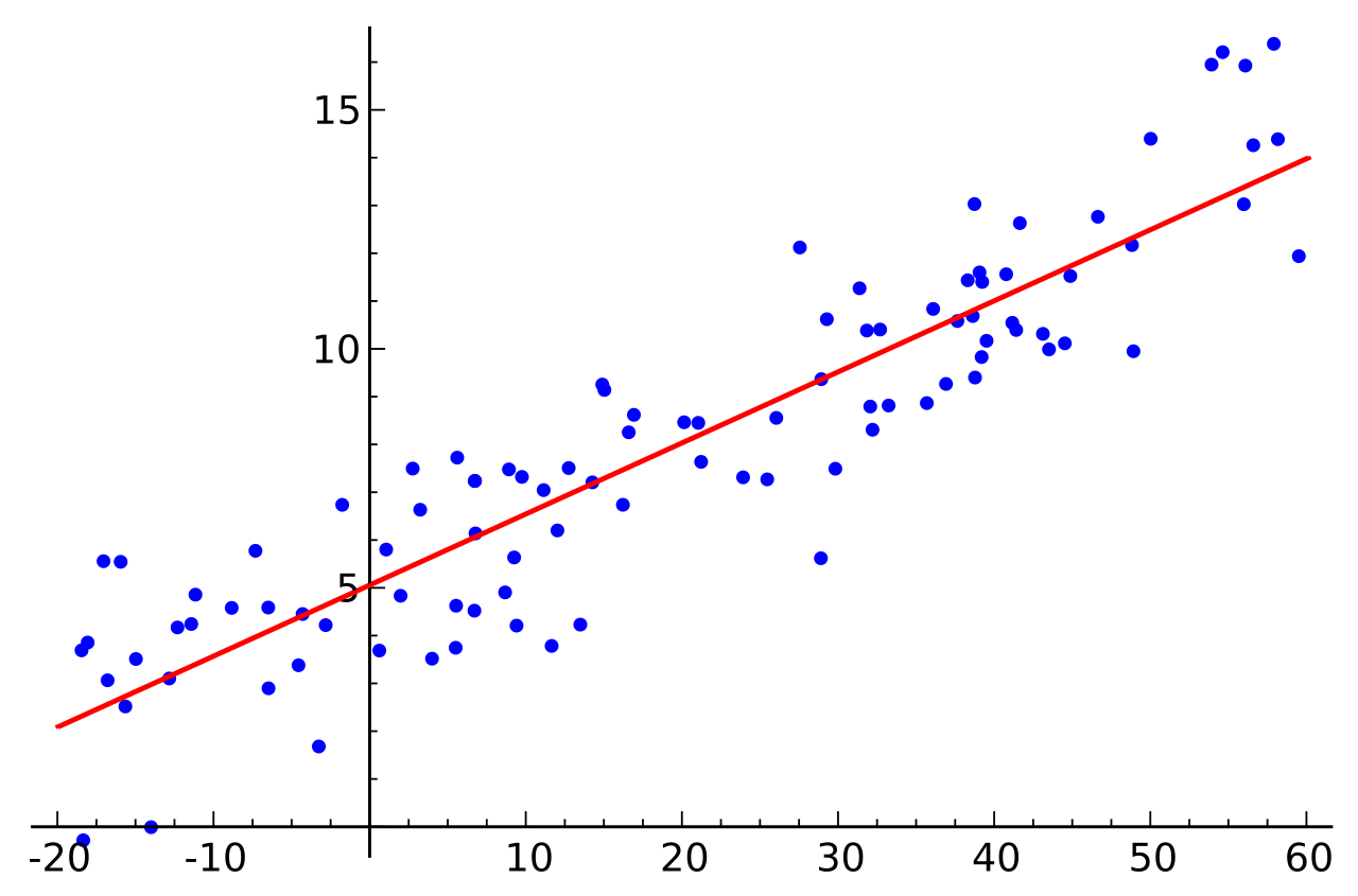
A scatterplot demonstrating a simple linear regression line, which acts as the model's best prediction for the trend of the bivariate data.

The standard equation of a linear regression line is written as:

$\hat{y} = a + bx$

Notice the "hat" over the $y$ . The variable $\hat{y}$ represents the predicted value of the response variable in a linear regression equation. It is vital to emphasize this to students: $\hat{y}$ is not the actual observed data point; it is the model's best guess for a given $x$ .

The Least-Squares Criterion

How do we decide where this line goes? We could eyeball it, but mathematics requires precision. We rely on the method of least squares.

The least-squares criterion minimizes the sum of the squares of the vertical distances of the data points from the regression line.

Think of the vertical distance between an actual data point and the regression line as an "error." By squaring these errors before adding them up, we accomplish two things: we treat positive and negative errors equally, and we heavily penalize large errors. Consequently, the line of best fit minimizes the sum of the squared residuals.

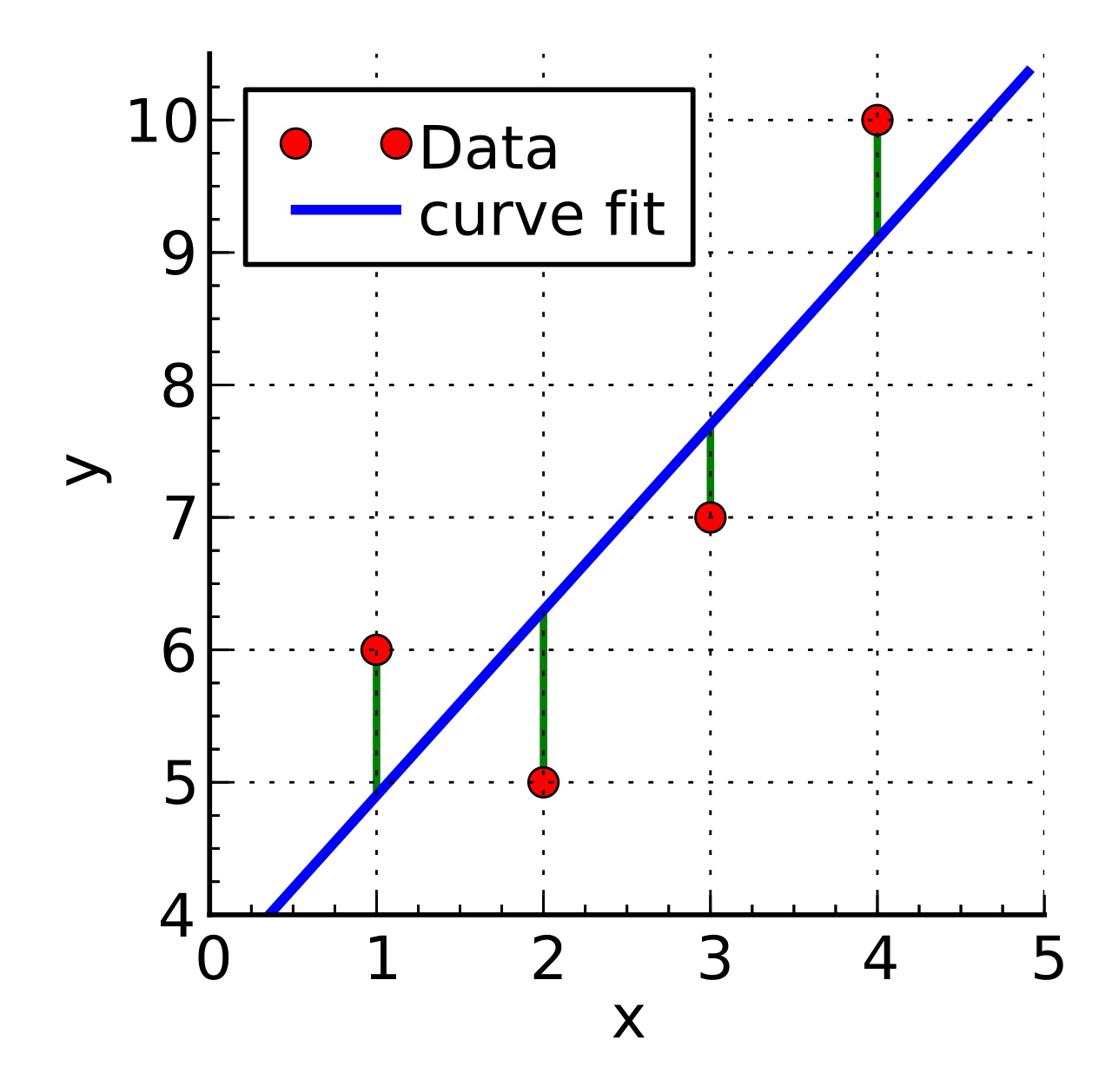
The least-squares regression line (blue) minimizes the squared vertical distances (green) between the actual observed data points (red) and the predicted values on the line.

The power of a regression line lies in its constants: the slope ( $b$ ) and the y-intercept ( $a$ ). These numbers are not arbitrary; they have precise physical or contextual meanings.

The slope of a regression line represents the predicted change in the response variable for a one-unit increase in the explanatory variable. If $x$ is "hours studied" and $y$ is "exam score," a slope of 4.5 means that for every additional hour a student studies, their predicted exam score increases by 4.5 points.
The y-intercept of a regression line represents the predicted value of the response variable when the explanatory variable is zero. In our studying example, this would be the predicted score for a student who studied for exactly zero hours.

To compute these parameters algebraically from summary statistics, we use two fundamental formulas:

The slope of the least-squares regression line equals the correlation coefficient multiplied by the ratio of the y standard deviation to the x standard deviation.

$b = r \cdot \frac{s_y}{s_x}$ This beautifully illustrates that the slope is simply the correlation ( $r$ ) scaled to the units of the data ( $s_y / s_x$ ).
The y-intercept of the least-squares regression line equals the mean y-value minus the product of the slope and the mean x-value.

$a = \bar{y} - b\bar{x}$

This second formula reveals a profound geometric truth: the least-squares regression line always passes through the point containing the mean of the x-values and the mean of the y-values, denoted as $(\bar{x}, \bar{y})$ . This point acts as a fulcrum, anchoring the regression line as it balances the data around it.

The Danger of Extrapolation

While our model is powerful, its jurisdiction is strictly limited to the domain of our data. Extrapolation occurs when a regression model predicts values outside the range of the observed explanatory variables.

If you build a regression line to predict reading speed based on the ages of elementary school children (ages 5 to 11), you cannot use that same line to predict the reading speed of a 45-year-old adult. The linear trend almost certainly flattens out or changes. Therefore, predictions made through extrapolation have a high risk of being inaccurate.

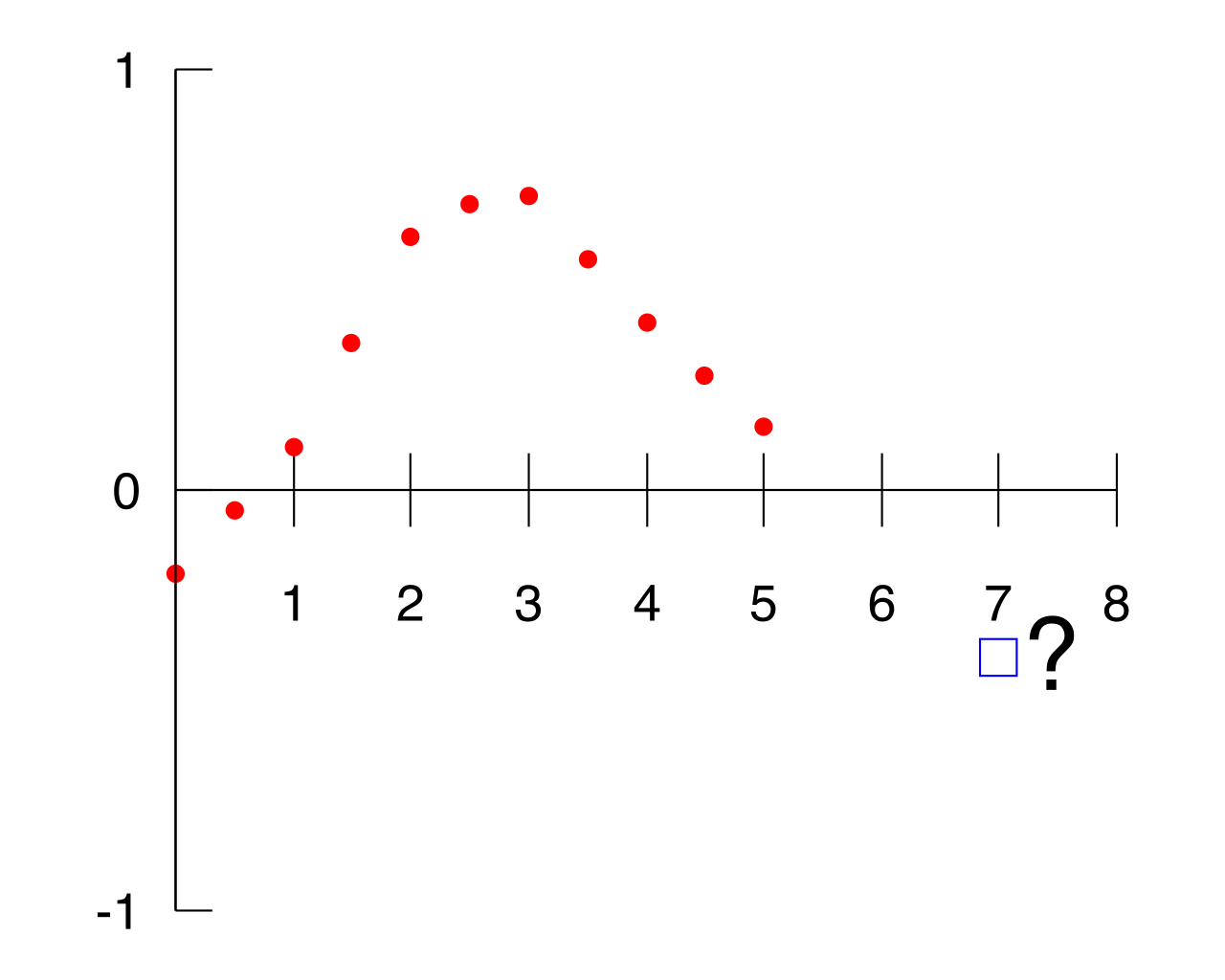
Predicting values outside the domain of the observed data (the red points) forces the model to assume the linear trend continues indefinitely, which often leads to inaccurate estimates (the blue box).

Before we even draw a line, we must determine if a linear relationship exists at all. This is the job of the Pearson correlation coefficient, denoted by $r$ .

The correlation coefficient $r$ measures the strength and indicates the direction of the linear relationship between two quantitative variables.

The value of the Pearson correlation coefficient $r$ always falls between -1 and 1 inclusive.

A correlation coefficient of exactly 1 indicates a perfect positive linear relationship. Every point lies exactly on an upward-sloping line.
A correlation coefficient of exactly -1 indicates a perfect negative linear relationship. Every point lies exactly on a downward-sloping line.
A correlation coefficient of zero indicates the absence of a linear relationship between the variables.

Structural Properties of the Correlation Coefficient

The correlation coefficient is remarkably resilient. Because it is calculated using standardized variables (z-scores), it is entirely unitless and immune to simple transformations:

Switching the explanatory variable and response variable does not change the value of the correlation coefficient. (If math score correlates to reading score at $0.8$ , reading score correlates to math score at $0.8$ ).
Adding a constant to all values of a variable does not change the correlation coefficient. If you curve an exam by adding 10 points to every student's score, the correlation with their attendance remains identical.
Multiplying all values of a variable by a positive constant does not change the correlation coefficient. If you track a student's study time in minutes rather than hours (multiplying by 60), $r$ remains unchanged.

Limitations: What $r$ Cannot Do

It is crucial to remember that the correlation coefficient only measures the strength of linear associations. It is entirely blind to curves. If you track the trajectory of a thrown baseball, the relationship between time and height is a perfect parabola. Yet, if you calculate $r$ for that data, you might get a value near zero. Therefore, the correlation coefficient cannot accurately measure the strength of non-linear associations.

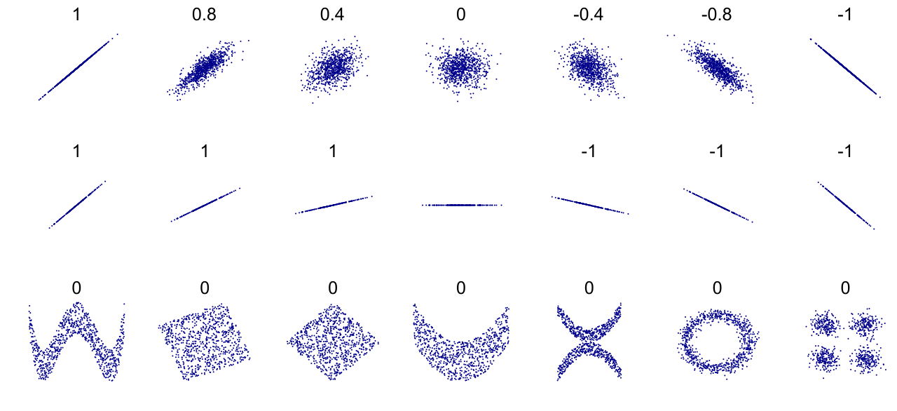
Various scatterplots and their corresponding Pearson correlation coefficients. Notice how the bottom row displays distinct non-linear patterns that have a correlation of exactly zero, demonstrating that the coefficient only measures linear relationships.

Furthermore, we must address the golden rule of statistics: A strong correlation between two variables does not guarantee a causal relationship.

Why? Because the real world is messy and interwoven with hidden factors.

Lurking variables can create a spurious correlation between two unrelated variables. For example, there is a strong positive correlation between a child's shoe size and their vocabulary. Does buying larger shoes teach a child more words? No. The lurking variable is age.
Similarly, a confounding variable is an unmeasured third variable influencing the supposed cause, and simultaneously, a confounding variable is an unmeasured third variable influencing the supposed effect. It entwines the variables so tightly that their individual effects cannot be untangled mathematically.

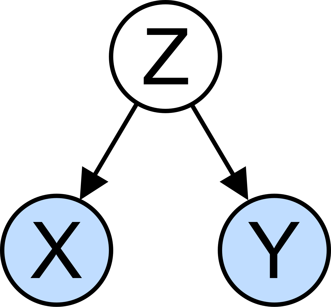
A confounding variable (Z) secretly influences both the supposed cause (X) and effect (Y), creating a spurious correlation that can easily be mistaken for direct causation.

If we want to prove that $x$ actually causes $y$ , observational data and correlation coefficients are never enough. Establishing causation requires a carefully designed randomized controlled experiment.

While $r$ gives us a standardized index of correlation, its square provides a much more intuitive, practical metric.

The coefficient of determination is calculated by squaring the Pearson correlation coefficient for a linear model ( $r^2$ ).

What does this number tell us? The coefficient of determination represents the proportion of the variance in the response variable predictable from the explanatory variable.

If the correlation between classroom attendance and final grades is $r = 0.8$ , then $r^2 = 0.64$ . This tells you that 64% of the variation in final grades can be explained by the variation in attendance. The remaining 36% of the variance is driven by other factors not captured by this specific model (like prior knowledge, test anxiety, or sleep).

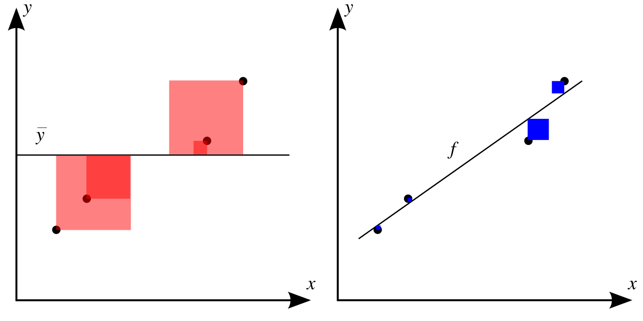
A visual representation of the coefficient of determination. The blue squares show the smaller squared errors of the linear regression model compared to the red squares, which represent the errors when simply using the average as a baseline.

A high $r^2$ does not automatically validate your linear model. To truly assess the fit of a function, we must interrogate the errors our model makes.

A residual is the difference between an observed value of the response variable and the predicted value from the regression line:

$\text{Residual} = y - \hat{y}$

A positive residual indicates the regression model underestimated the actual observed value. (The point lies above the regression line).
A negative residual indicates the regression model overestimated the actual observed value. (The point lies below the regression line).

By mathematical design, the least-squares process balances these errors perfectly. Therefore, the sum of the residuals for any least-squares regression line is exactly zero.

Reading the Residual Plot

To diagnose our model, we construct a specific graph. A residual plot is a scatterplot displaying the explanatory variable on the horizontal axis and the corresponding residuals on the vertical axis. It acts like an x-ray, removing the overarching linear trend so we can inspect the underlying structure of the errors.

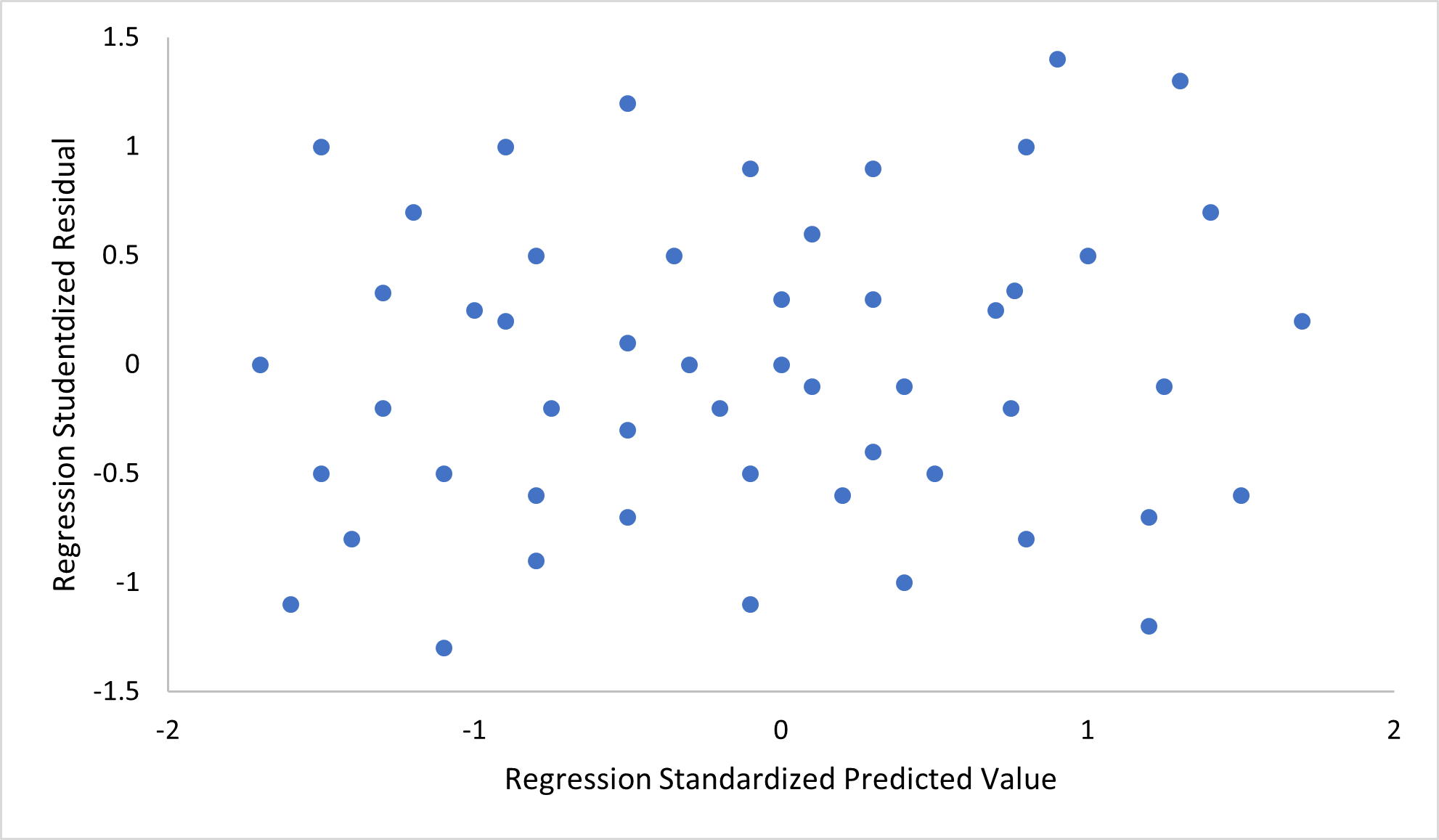
An ideal residual plot exhibits a random scatter of points around the zero line, indicating that the linear model has successfully captured the underlying trend without leaving systemic patterns behind.

Pattern Observed in Residual Plot	Interpretation for the Model
Random scatter above and below the zero-line	A residual plot showing a random scatter of points around the horizontal axis indicates a linear model is appropriate. The model captured the signal; only random noise is left.
U-shape or inverted U-shape	A distinct curved pattern in a residual plot indicates a non-linear model would better fit the data. The linear model failed to capture a curving trend.
Fan or Megaphone shape	Increasing variance of residuals across the horizontal axis of a residual plot indicates heteroscedasticity. The model is highly accurate for low values of $x$ , but becomes wildly inaccurate for high values of $x$ (or vice versa).

Finally, what happens when a single student's data deviates wildly from the class? In regression analysis, we classify unusual points based on how they deviate and the impact they have on the model.

Outliers: An outlier in a regression context is a data point with a remarkably large absolute residual. It sits very far above or below the regression line, meaning the model's prediction for that point is terribly wrong.
High Leverage: Think of the regression line like a seesaw, with the fulcrum at the mean of x ( $\bar{x}$ ). Data points located far away from the center have immense mechanical advantage. Therefore, points with high leverage have x-values situated far from the mean of the x-values. They have the potential to drastically alter the line.
Influential Points: When a point actually exercises that leverage to pull the line toward itself, it becomes influential. An influential point is a data observation causing a significant change in the slope of the regression line upon removal, as well as an influential point is a data observation causing a significant change in the y-intercept of the regression line upon removal.

If you have a student who barely studies but achieves a perfect score, they might be an outlier. But if you have a student who studies for 40 hours (far exceeding the class average of 5 hours) and scores very poorly, they have high leverage. If removing that single student's data drops your regression line's slope from $0.8$ to $0.2$ , that student is undeniably an influential point.

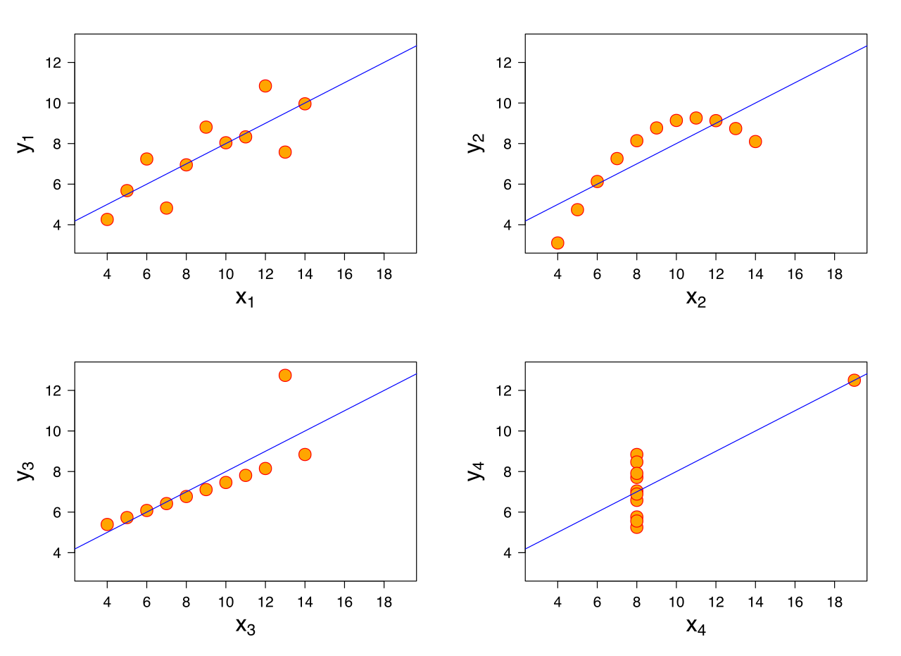
Anscombe's quartet demonstrates the danger of relying solely on summary statistics. The bottom right graph features a highly influential point with extreme leverage that completely dictates the slope of the regression line.

By mastering these concepts, you equip yourself not just to calculate formulas, but to interpret the stories hidden within data—an invaluable skill for any modern educator.