Simple and Compound Probability
Not sure you’re ready?
Take the ~3-minute readiness diagnostic and see where you stand.
When a student reaches into a bag of assorted colored tiles to draw one at random, they are not merely playing a game; they are interrogating a meticulously defined universe of mathematical outcomes. The mathematics of probability provides a rigorously structured language for measuring uncertainty, a critical tool in fields ranging from quantum mechanics to actuarial science. For the aspiring secondary mathematics educator, mastering probability is about far more than calculating dice rolls or passing the Praxis 5165. It is about equipping your future students to navigate a world inundated with risk assessments, medical testing statistics, and predictive algorithms. We must move them past intuition—which is notoriously flawed when it comes to chance—and ground them in the structural logic of sample spaces, conditional events, and independence.
Let us build the foundation of theoretical probability from the ground up, ensuring you possess both the rigorous definitions required for the exam and the intuitive framing necessary for the classroom.
Before we can determine the likelihood of an outcome, we must define the universe in which we are operating. In probability, this universe is called the sample space.
The sample space of a probabilistic experiment is the set of all possible outcomes.
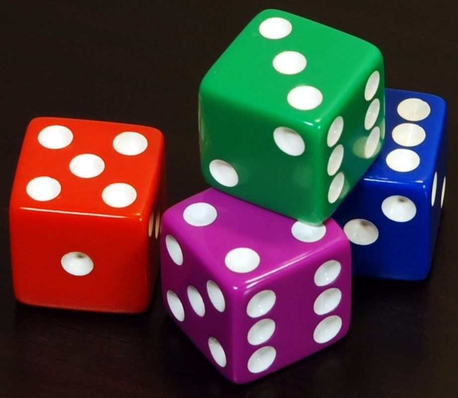
If you are rolling a standard six-sided die, the sample space S is {1,2,3,4,5,6}. Once the universe is established, we can define the specific occurrences we care about. An event is defined mathematically as a subset of the sample space. If our event A is "rolling an even number," then A={2,4,6}.
In many introductory scenarios, we rely on a uniform probability model. In a uniform probability model, all outcomes in the sample space are equally likely to occur. When rolling a fair die, each face has an identical chance of landing face up. Because of this symmetry, the probability of an event in a uniform probability model is the number of outcomes in the event divided by the total number of outcomes in the sample space.
For our even-number event A, there are 3 outcomes in the event and 6 in the total sample space, yielding P(A)=63=21.
When teaching this, emphasize the fundamental boundaries that govern these calculations. Because an event cannot have fewer than zero outcomes, nor can it have more outcomes than the sample space itself, the probability of any event must be a real number between 0 and 1, inclusive. An impossible event has a probability of 0, and a guaranteed event has a probability of 1. Furthermore, if you evaluate every distinct, non-overlapping possibility in your universe, the sum of the probabilities of all distinct outcomes in a sample space equals exactly 1. You are distributing exactly 100% of the certainty across the possible outcomes.
Events rarely exist in isolation. Students will frequently encounter situations where multiple conditions are tested simultaneously. To navigate this, we map probability directly onto set theory.
The Complement
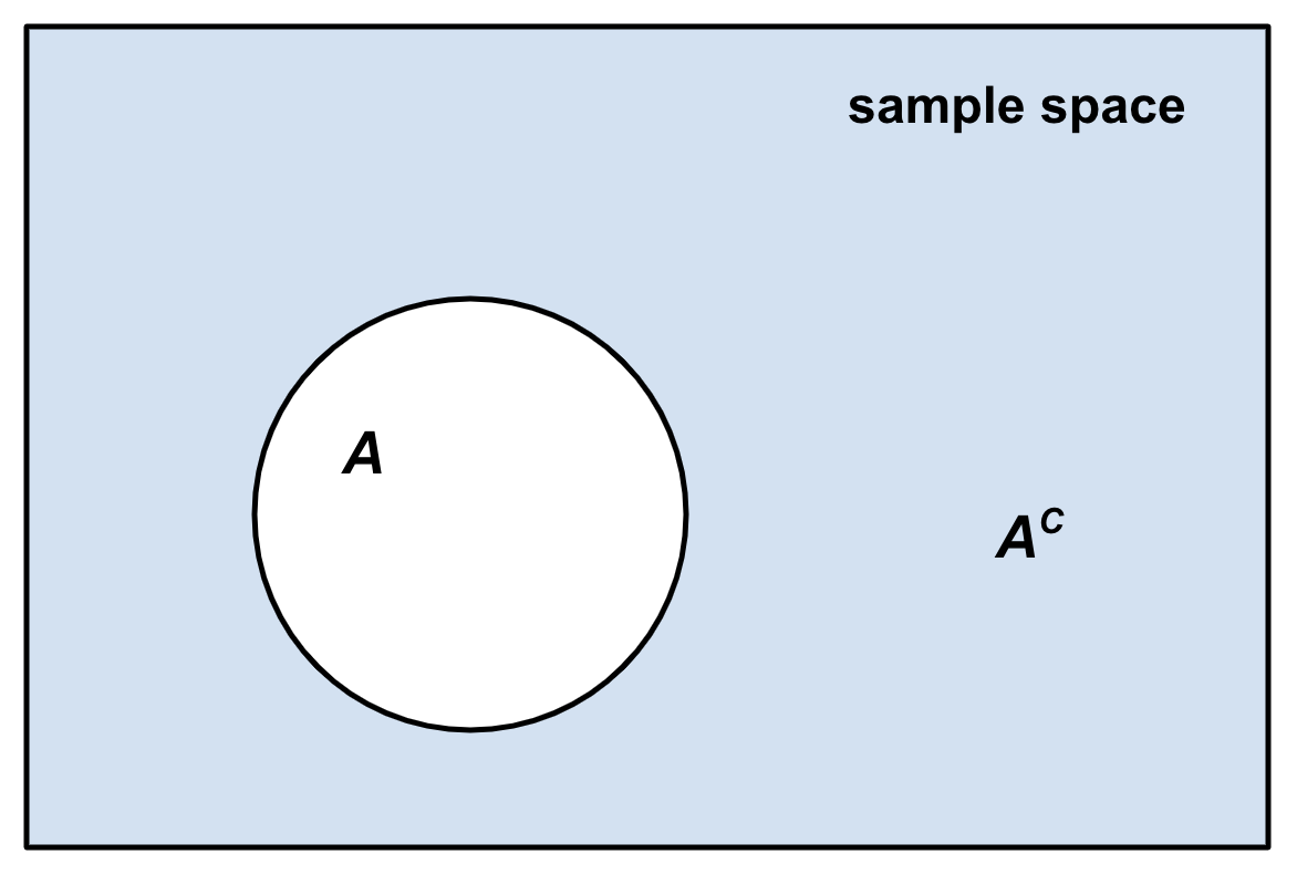
Sometimes, it is mathematically simpler to calculate the probability of what did not happen than what did. The complement of an event A contains all outcomes in the sample space that are not in event A. Denoted as A′ or Ac, the complement represents the "everything else." Because the event and its complement perfectly partition the sample space, their probabilities must sum to 1. Therefore, the probability of the complement of an event A is equal to 1 minus the probability of event A.
Unions and Intersections
Consider two events, A and B.
- The intersection of two events A and B contains only the outcomes that are simultaneously in both event A and event B. This is the logical "AND", representing the overlap in a Venn diagram.
- The union of two events A and B contains all outcomes that are in event A, in event B, or in both events. This is the logical "OR".
How do we calculate the probability of the union? Your students' first instinct will be simply to add the probability of A to the probability of B. But nature has a way of balancing the books. If we simply add P(A) and P(B), we double-count the intersection where the two events overlap. We must subtract that intersection to correct the tally.
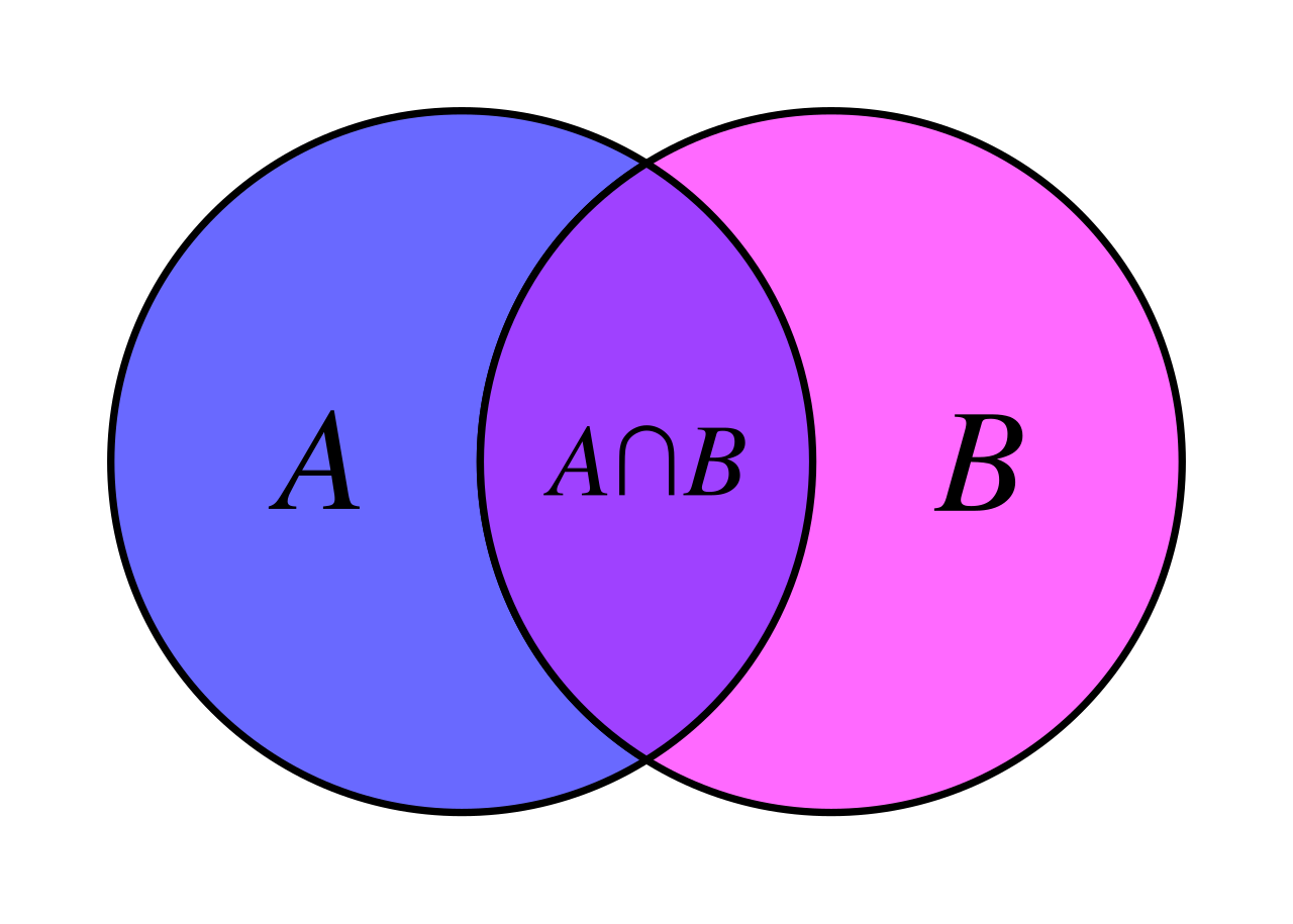
This correction gives us the most important formula in basic set probability:
The General Addition Rule: The probability of event A union event B equals the probability of event A plus the probability of event B minus the probability of event A intersection event B. P(A∪B)=P(A)+P(B)−P(A∩B)
Mutually Exclusive Events
What if there is no overlap to subtract? Suppose event A is "rolling a 2" and event B is "rolling a 3." You cannot roll a 2 and a 3 on a single die at the same time.
Two events are mutually exclusive if the intersection of the two events is the empty set. Practically speaking, mutually exclusive events cannot occur at the same time. Because their intersection is the empty set, the probability of their intersection is 0.
Consequently, the General Addition Rule simplifies beautifully: The probability of the union of two mutually exclusive events is the sum of the individual probabilities of those events. P(A∪B)=P(A)+P(B)
One of the most fascinating aspects of probability—and a concept that fundamentally governs statistical machine learning and medical diagnostics—is how the introduction of new information alters our assessment of chance.
Conditional probability is the probability of an event A occurring given that a second event B has already occurred. The notation P(A∣B) is read as "the probability of A, given B."
When we are given B, we are effectively shrinking our universe. The original sample space no longer matters; we only care about the subset of outcomes where B has occurred. To find the probability of A within this new, shrunken universe, we look at the overlap of A and B, and divide it by our new total universe, B.
Formula for Conditional Probability: The conditional probability of event A given event B is calculated by dividing the probability of the intersection of events A and B by the probability of event B. P(A∣B)=P(B)P(A∩B)
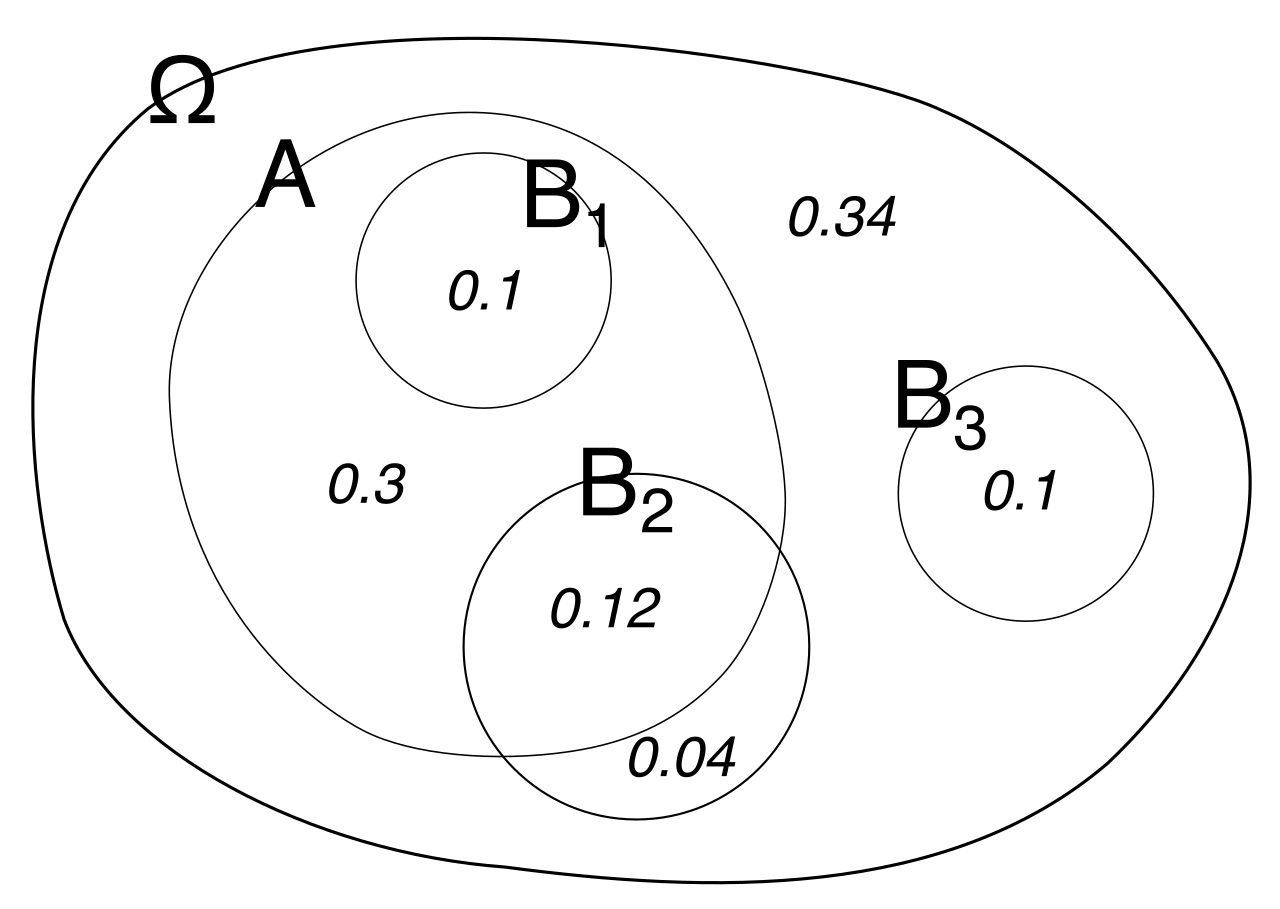
If we rearrange this algebraic relationship by multiplying both sides by P(B), we generate a powerful tool for calculating the probability of a sequence of events.
The General Multiplication Rule: The probability of the intersection of events A and B equals the probability of event A multiplied by the conditional probability of event B given event A. P(A∩B)=P(A)⋅P(B∣A)
Independence versus Dependence
In the physical classroom, you will frequently model probability by pulling objects from a container—say, drawing student names from a hat to form presentation groups.
If you draw a student's name, read it, and leave it out of the hat, the sample space for the next draw has changed. The first event has fundamentally altered the probability of the second. Sampling items from a finite population without replacement generally results in dependent events.
However, if you draw a name, read it, and place it back into the hat, the sample space is entirely restored. The universe resets. Sampling items from a population with replacement generally results in independent events.
This brings us to the formal definition of independence. Two events are independent if the occurrence of one event does not change the probability of the occurrence of the other event.
Mathematically, this concept provides us with two rigorous test conditions for independence:
- Two events A and B are independent if and only if the conditional probability of event A given event B equals the marginal probability of event A. P(A∣B)=P(A) (Meaning: Knowing that B happened provided absolutely no mathematical information that altered the likelihood of A).
- Two events A and B are independent if and only if the probability of the intersection of A and B equals the product of the individual probabilities of A and B. P(A∩B)=P(A)⋅P(B) (This flows directly from substituting P(A) for P(A∣B) in the General Multiplication Rule).
If either of these conditions fails, the events are dependent.
Probability can quickly become an abstract soup of algebraic notation. To ground these concepts, mathematics curricula heavily emphasize tabular representations. A two-way frequency table displays the joint frequencies of two categorical variables. It is a brilliant teaching tool because it makes the "shrunken universe" of conditional probability visually explicit.
Imagine surveying 200 high school students about whether they are taking a foreign language, categorized by grade level.
| Taking Language | Not Taking Language | Row Totals | |
|---|---|---|---|
| Juniors | 50 | 30 | 80 |
| Seniors | 40 | 80 | 120 |
| Column Totals | 90 | 110 | 200 |
Navigating the Table: Margins and Joints
The numbers inside the main body of the table (50, 30, 40, 80) are joint frequencies. The numbers on the edges (80, 120, 90, 110) are marginal frequencies.
Notice the physical construction of the data: A marginal frequency in a two-way table is calculated by summing a single row or a single column of joint frequencies. (e.g., 50+30=80 Juniors total).
If we divide these frequencies by the grand total (200), we convert raw counts into probabilities, generating a relative frequency table.
- A joint relative frequency in a two-way table represents the probability of the intersection of two specific categories. The probability that a randomly selected student is a Junior AND taking a language is 20050=0.25.
- A marginal relative frequency in a two-way table represents the probability of a single category without considering the other categorical variable. The probability that a randomly selected student is a Junior, regardless of language status, is 20080=0.40.
Conditional Probability and Independence in Tables
Two-way tables make the formula for conditional probability trivial to execute. If we want to find the probability that a student is taking a language given that they are a Junior, P(Language∣Junior), we restrict our universe solely to the Junior row. The total universe is now 80. The number of those 80 who fit our criteria is 50.
Thus, P(Language∣Junior)=8050=0.625.
Notice what we just did mathematically: A conditional probability can be estimated from a two-way frequency table by dividing a specific joint frequency by the corresponding marginal frequency. We divided the joint frequency (50) by the marginal frequency of the condition (80).
Finally, we can use these tables to investigate independence. Does being a Junior impact the likelihood of taking a language?
- Conditional probability: P(Language∣Junior)=0.625
- Marginal probability: P(Language)=20090=0.450
Because 0.625=0.450, the events are dependent. Grade level clearly impacts the decision to take a language. Independence between two categorical variables can be tested by checking if a conditional relative frequency equals the corresponding marginal relative frequency in a two-way table.
When you sit for the Praxis 5165, you will be expected to toggle effortlessly between reading a dense word problem and identifying whether a scenario demands an intersection, a conditional probability, or a test for independence. Graphing calculators can assist with massive sample space factorials and combinatorics, but the logic of simple and compound probability is entirely structural.
Teach your students to identify the "ANDs," the "ORs," and the "GIVENs." Teach them to map formulas onto Venn diagrams and two-way tables. When they can visualize the universe of possible outcomes expanding and contracting based on the given information, probability ceases to be a list of memorized formulas and becomes exactly what it is: the eloquent geometry of chance.