Polynomial Functions and Zeros
Not sure you’re ready?
Take the ~3-minute readiness diagnostic and see where you stand.
When a structural engineer models the load on a suspension bridge, or a data scientist fits a curve to fluctuating market trends, they rely on a mathematical armature: the polynomial function. For your secondary students, however, a polynomial of degree n often looks like an arbitrary string of algebraic symbols. As a mathematics educator, your objective is to teach them to read this equation like a genetic sequence. Every intersection with the axes, every peak and valley, and the ultimate trajectory of the curve to infinity is pre-encoded in its coefficients and degree.
To translate between the algebraic expression and the geometric curve, we must systematically dismantle the polynomial into its fundamental building blocks: its linear factors. In mastering these principles for the Praxis 5165 exam, you are not merely reviewing algebra; you are refining the pedagogical tools you will use to help students bridge the abstract manipulation of variables with the concrete visualization of space.
Before a student can sketch a curve, they must locate its anchors. We begin with the concept of a root.
The roots of a polynomial function correspond exactly to the input values where the polynomial evaluates to zero.
Finding these roots algebraically relies on our ability to factor the polynomial, which rests entirely on a single, powerful piece of logic:
The zero product property is the algebraic principle that if a product of factors equals zero, at least one of the factors must equal zero.
When you hand a student an expanded polynomial like P(x)=x3−4x2+x+6, they cannot immediately see the zeros. They must divide to find factors. But polynomial long division is notoriously cumbersome and prone to arithmetic errors. Enter our first major shortcut.
The Remainder and Factor Theorems
The Remainder Theorem states that dividing a polynomial P(x) by a linear binomial x−c results in a remainder equal to P(c).
This theorem is profound because it establishes an equivalence between division and evaluation. If a student wants to know what P(5) is, they don't have to calculate 53−4(52)+5+6; they can simply divide P(x) by x−5 and look at the remainder.
To execute this division efficiently, we use a streamlined algorithm.
Synthetic division is an algorithmic process used to divide a polynomial by a linear binomial of the form x−c.
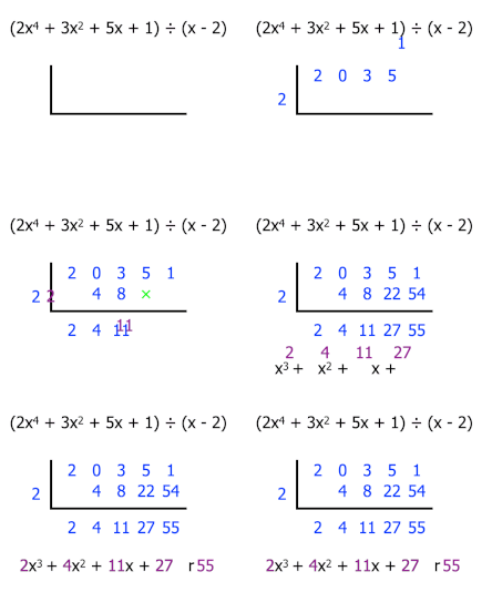
By stripping away the variables and working only with coefficients, synthetic division accelerates the division process. Because of the Remainder Theorem, we know that:
The numerical remainder obtained from synthetic division of a polynomial by x−c is equal to the value of the polynomial function evaluated at x=c.
This brings us to the ultimate goal of factorization. If the remainder is exactly zero, it means P(c)=0. Therefore, c is a root, and x−c perfectly divides the polynomial.
The Factor Theorem states that a polynomial P(x) has a factor of x−c if and only if the polynomial evaluated at c equals zero.
As a teacher, you will rely on the Factor Theorem daily to reverse-engineer test questions. If you want an exam problem to have roots at x=2 and x=−3, you multiply (x−2) and (x+3) to build the polynomial.
How many roots should a student look for? If they find two roots for a cubic function, are they finished?
The Fundamental Theorem of Algebra
The Fundamental Theorem of Algebra guarantees that every non-zero single-variable polynomial with complex coefficients has at least one complex root.
By iteratively applying the Fundamental Theorem of Algebra and the Factor Theorem, we arrive at a strict accounting rule for the total number of zeros in a system:
A polynomial of degree n has exactly n complex roots when accounting for the multiplicity of each root.
Narrowing the Search Field
Telling a student a 4th-degree polynomial has exactly 4 complex roots gives them a target, but it doesn't tell them where to start testing values via synthetic division. Instead of guessing blindly across the infinite number line, we teach them to use predictive theorems to generate a finite list of candidates.
The Rational Root Theorem states that any rational root of a polynomial must be a ratio of an integer factor of the constant term to an integer factor of the leading coefficient.
If P(x)=2x3+⋯−15, your students only need to test ratios constructed from the factors of −15 (numerator) and 2 (denominator).
Furthermore, we can predict the nature of the real roots.
Descartes' Rule of Signs calculates the possible number of positive real roots of a polynomial based on the number of sign changes in the polynomial's consecutive non-zero coefficients.
(Note: Evaluating P(−x) and counting sign changes provides the possible number of negative real roots).
Missing Roots: The Conjugate Theorems
Sometimes, the Rational Root Theorem yields no real answers, or synthetic division leaves us with an irreducible quadratic. When we turn to the quadratic formula, irrational and complex roots emerge, and they never arrive alone.
The Complex Conjugate Root Theorem states that if a polynomial with real coefficients has a complex root a+bi, then the complex conjugate a−bi is also a root of that polynomial.
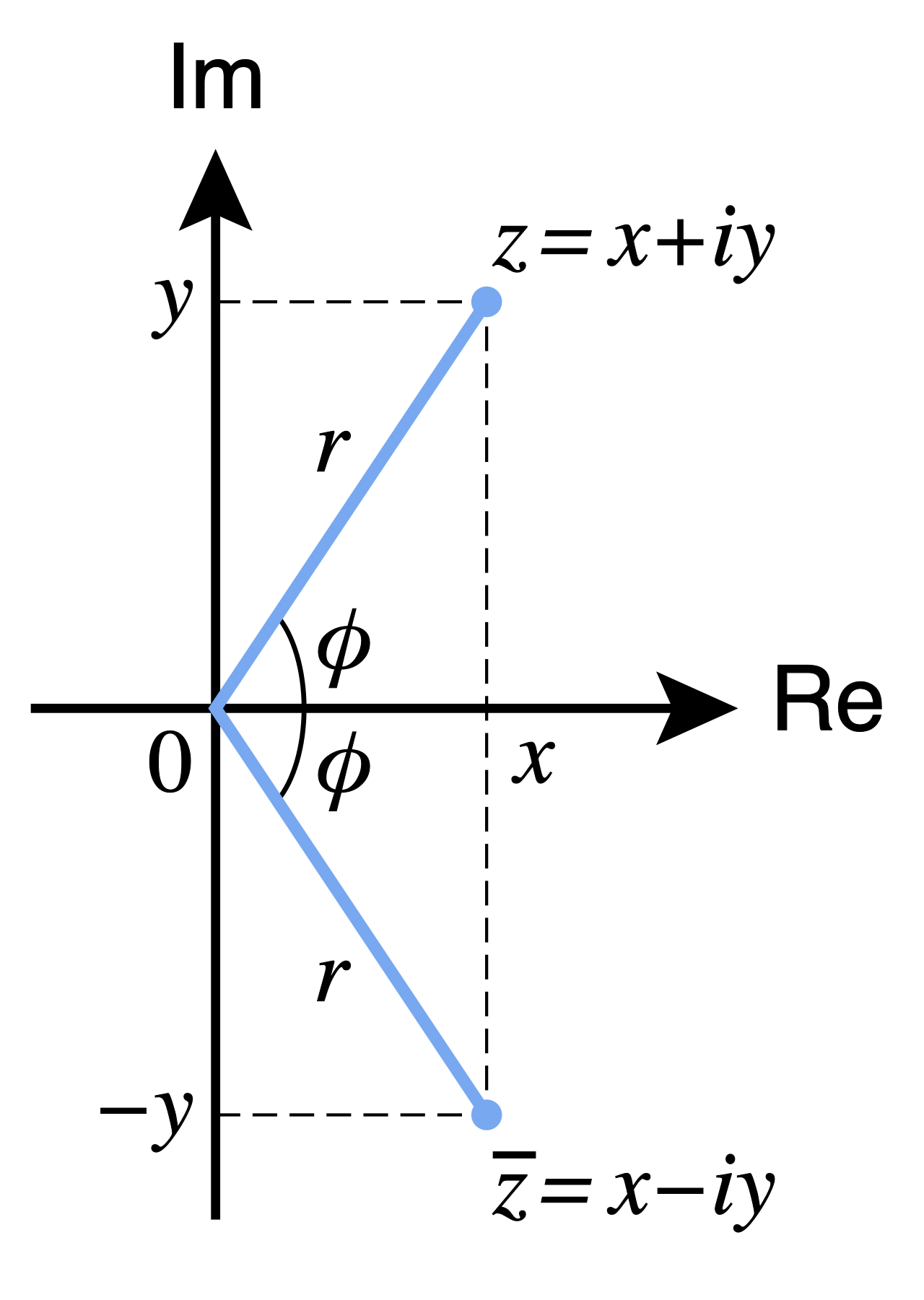
Similarly, symmetry exists for irrational roots:
The Irrational Conjugate Root Theorem states that if a polynomial with rational coefficients has a root a+b, then a−b is also a root.
For your Praxis exam—and your future lesson planning—this means if you are given a 3rd-degree polynomial with real coefficients, and you know x=2 and x=3i are roots, the third root must be −3i.
Once the roots are found, we transition from algebraic manipulation to Cartesian geometry. We must show students how the numbers dictate the shape of the curve.
Intercepts: Real vs. Complex
A common student misconception is that all roots appear as x-intercepts. As an educator, you must clarify the geometric boundaries of the x,y-plane:
Real zeros of a polynomial function correspond precisely to the x-intercepts of the function's graph on the Cartesian coordinate plane.
However, the coordinate plane only plots real numbers. Therefore:
Complex zeros with non-zero imaginary parts do not produce x-intercepts on the Cartesian coordinate plane.
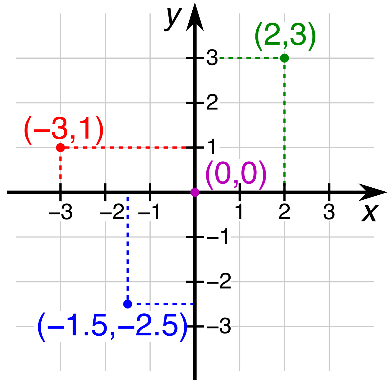
While the x-intercepts require significant algebraic heavy lifting to uncover, the y-intercept is a simple matter of evaluation.
The y-intercept of a polynomial function is determined by evaluating the function at x=0.
Because substituting 0 eliminates every term containing the variable x, we arrive at a universally helpful shortcut for graphing:
The y-intercept of a polynomial function is mathematically equivalent to the constant term of the polynomial expression.
End Behavior: The Infinite Horizon
Before drawing the middle of the curve, we must establish where it begins and ends.
The end behavior of a polynomial graph describes the direction the graph heads as the x-values approach positive infinity and negative infinity.
When x becomes massively large (positive or negative), the term with the highest exponent dominates all other terms. Therefore:
The end behavior of a polynomial function is determined jointly by the polynomial's degree and the sign of the polynomial's leading coefficient.
You should train your students to recognize the four possible quadrants of end behavior, conceptualizing them as generalizations of the basic parabola (x2) and cubic (x3) graphs.
| Degree | Leading Coefficient | Left Behavior (x→−∞) | Right Behavior (x→∞) | Formal Definition |
|---|---|---|---|---|
| Even | Positive (+) | Approaches +∞ | Approaches +∞ | > A polynomial function with an even degree and a positive leading coefficient approaches positive infinity as x approaches both positive infinity and negative infinity. |
| Even | Negative (−) | Approaches −∞ | Approaches −∞ | > A polynomial function with an even degree and a negative leading coefficient approaches negative infinity as x approaches both positive infinity and negative infinity. |
| Odd | Positive (+) | Approaches −∞ | Approaches +∞ | > A polynomial function with an odd degree and a positive leading coefficient approaches negative infinity as x approaches negative infinity and positive infinity as x approaches positive infinity. |
| Odd | Negative (−) | Approaches +∞ | Approaches −∞ | > A polynomial function with an odd degree and a negative leading coefficient approaches positive infinity as x approaches negative infinity and negative infinity as x approaches positive infinity. |
Multiplicity: Navigating the Intersections
We know the ends of the graph, and we know exactly where it touches the x-axis. But how does it interact with the axis? The behavior at an x-intercept is entirely governed by how many times that specific root is duplicated.
The multiplicity of a polynomial zero is the number of times the zero's corresponding linear factor appears in the completely factored form of the polynomial.
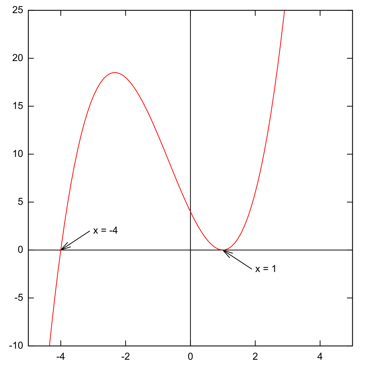
If a polynomial factors into P(x)=(x−2)3(x+4)2(x−7)1, the root x=2 has a multiplicity of 3, x=−4 has a multiplicity of 2, and x=7 has a multiplicity of 1. The parity (odd or even) of the multiplicity determines the local geometry:
Odd Multiplicity:
A real zero with an odd multiplicity causes the polynomial graph to cross the x-axis at that specific x-value.
We can refine this further based on the specific odd integer:
- Multiplicity of 1: > A real zero with a multiplicity of exactly 1 produces a straight crossing of the x-axis. (It looks locally like a linear function).
- Multiplicity of 3, 5, 7...: > A real zero with an odd multiplicity greater than 1 causes the polynomial graph to flatten out as the graph crosses the x-axis at that specific x-value. (It looks locally like a cubic inflection).
Even Multiplicity:
A real zero with an even multiplicity causes the polynomial graph to touch the x-axis and turn around without crossing to the other side of the x-axis. (It looks locally like a parabola bouncing off the axis).
Turning Points: The Local Extrema
Finally, as the graph weaves through these x-intercepts, obeying its multiplicity rules and marching toward its predetermined end behavior, it must change direction.
A turning point on a polynomial graph is a local maximum or local minimum where the graph changes from increasing to decreasing or from decreasing to increasing.
Because a polynomial is a continuous, smooth curve, the maximum number of times it can change direction is directly constrained by its degree:
A polynomial function of degree n has a maximum of n−1 turning points on its graph.
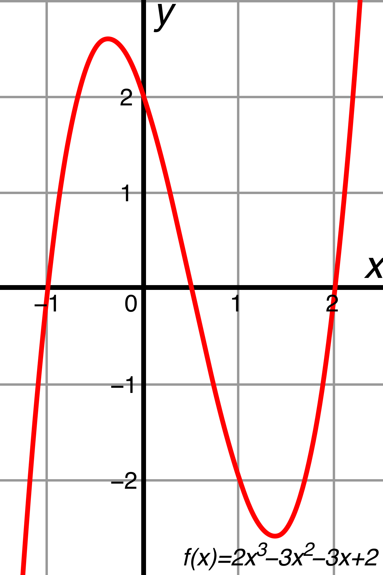
It is critical to note for your exam that a polynomial may have fewer than n−1 turning points (for instance, y=x3 has zero turning points), but it can never exceed this limit.
When you approach a selected-response or numeric-entry item on the Praxis 5165, view the problem structurally. If an item provides a graph that bounces at x=−1, crosses flatly at x=2, and goes from top-left to bottom-right, you immediately possess the entire algebraic skeleton:
- Top-left to bottom-right: Odd degree, negative leading coefficient.
- Bounce at x=−1: Factor of (x+1) with an even power (e.g., squared).
- Flat cross at x=2: Factor of (x−2) with an odd power >1 (e.g., cubed).
- y-intercept: Check where the curve crosses the y-axis to solve for the specific scalar multiplier (the leading coefficient a).
By internalizing these definitions not as isolated facts, but as an interconnected logical system, you transform polynomial analysis from rote memorization into a robust, elegant framework. This is the exact conceptual clarity you will soon impart to your own students.