Rational and Radical Equations

Not sure you’re ready?

Take the ~3-minute readiness diagnostic and see where you stand.

In algebraic manipulation, equality is a fragile state. When we perform operations on an equation, we operate under the fundamental assumption that we are walking a reversible path—that every step taken forward can be perfectly traced backward. However, certain mathematical operations act as one-way doors. By multiplying by variables or raising expressions to even powers, we inadvertently alter the foundational limits of the equation. We expand its domain, and in this newfound, broader space, mathematical "ghosts" can materialize. These ghosts are algebraically valid within the new structure but entirely false in the original. To master—and to successfully teach—rational and radical equations, one must understand not just the mechanics of solving them, but the deep structural reasons why these equations spontaneously generate illusions.

The first recorded use of the equals sign (1557). Establishing a statement of equality creates a fragile mathematical state that must be carefully preserved during manipulation.

Before we can solve equations, we must understand the objects that compose them. A rational expression is defined as the algebraic ratio of two polynomial expressions. Think of it as a fraction, but rather than dealing with static integers, we are dealing with dynamic functions.

The moment we construct a fraction, we introduce a strict boundary condition. Division by zero is undefined in the real number system. Consequently, the domain of a rational expression excludes any real number that evaluates to zero in the denominator. When you hand a rational expression to a student, you are handing them a machine with specific operating limits.

Handheld calculators explicitly throw errors when asked to divide by zero, visually reinforcing to students that rational expressions possess strict boundary conditions.

Rewriting and Simplifying

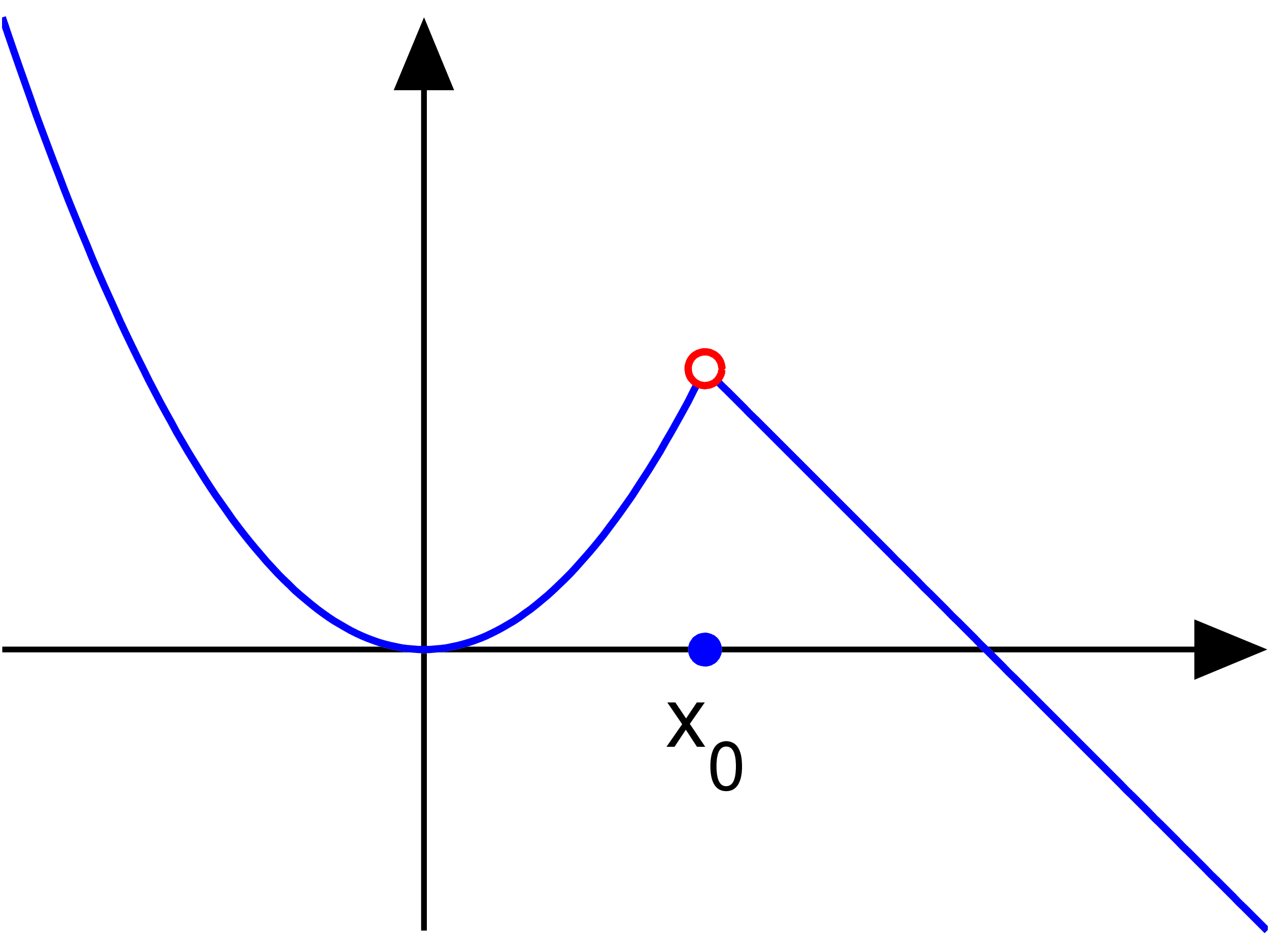
To simplify these expressions, we must factor the polynomials. Simplifying a rational expression requires dividing out the common factors shared by the numerator and the denominator. However, a critical pedagogical trap lies here. If you start with $f(x) = \frac{(x-3)(x+2)}{x-3}$ and simplify it to $g(x) = x+2$ , these functions are not identical everywhere.

Crucial Rule of Equivalence: The domain of a simplified rational expression must explicitly exclude values that made the original unsimplified denominator zero. Even though the $(x-3)$ factor was divided out, the domain of the simplified expression remains $x \neq 3$ .

The Arithmetic Operations

When teaching operations on rational expressions, your students already have the cognitive framework from elementary fractions. Your job is to activate it algebraically.

Operation	The Mechanism	Pedagogical Watch-Out
Multiplication	The product of two rational expressions is a new fraction containing the product of the original numerators divided by the product of the original denominators.	Students may over-complicate by trying to find common denominators unnecessarily. Factor first, multiply straight across, divide out common factors.
Division	Dividing one rational expression by another requires multiplying the first rational expression by the reciprocal of the second rational expression.	Remind students that reciprocating the second fraction introduces a new denominator, generating an additional domain restriction.
Addition & Subtraction	Adding (or subtracting) rational expressions requires rewriting the expressions to have a common denominator.	A common student error when adding rational expressions involves mistakenly adding the denominators together (e.g., $\frac{1}{x} + \frac{1}{y} = \frac{2}{x+y}$ ).

To successfully add or subtract, students must find the least common denominator (LCD), which is the least common multiple of all the polynomial denominators. Finding the LCD prevents the numerator from inflating into an unmanageable polynomial.

An equation is a statement that two expressions are equal. Rational equations can be simplified by multiplying every term on both sides by the least common denominator. This elegant maneuver clears the fractions entirely, transforming a complex rational equation into a familiar linear or quadratic one. Furthermore, if you encounter rational equations structured as a proportion between two fractions, they can be solved using cross-multiplication.

But this algebraic elegance comes at a steep price.

The Birth of Extraneous Solutions

Multiplying both sides of a rational equation by a variable expression can introduce extraneous solutions. Why does this happen?

Extraneous solutions occur when an applied mathematical operation creates a new equation with a broader domain than the original equation. Imagine the equation $\frac{x^2}{x-2} = \frac{4}{x-2}$ . The domain strictly prohibits $x = 2$ . However, if we multiply both sides by $(x-2)$ , we are left with $x^2 = 4$ , which is a standard polynomial. Polynomials have domains of all real numbers. The new equation has "forgotten" the restrictions of the original equation. Solving $x^2 = 4$ yields $x = 2$ and $x = -2$ .

Because $x=2$ causes the original denominator to evaluate to zero, it is a mathematical ghost. An extraneous solution to a rational equation is an algebraically derived value that causes a denominator in the original equation to evaluate to zero.

The Graphical Perspective

As a teacher preparing students for a technologically rich world, you must bridge the algebraic and the graphical. Graphing calculators identify real solutions to an equation by locating the x-coordinates of the intersection points of the left and right side functions.

When a student graphs the two sides of a rational equation, the extraneous solution will absolutely not yield an intersection point. Why? Because graphical representations of rational equations exclude extraneous solutions by displaying vertical asymptotes at invalid x-values, or, in cases where factors perfectly cancel out, graphical representations of rational equations exclude extraneous solutions by displaying removable discontinuities (holes) at invalid x-values. The calculator "sees" the domain restriction that the algebra "forgot."

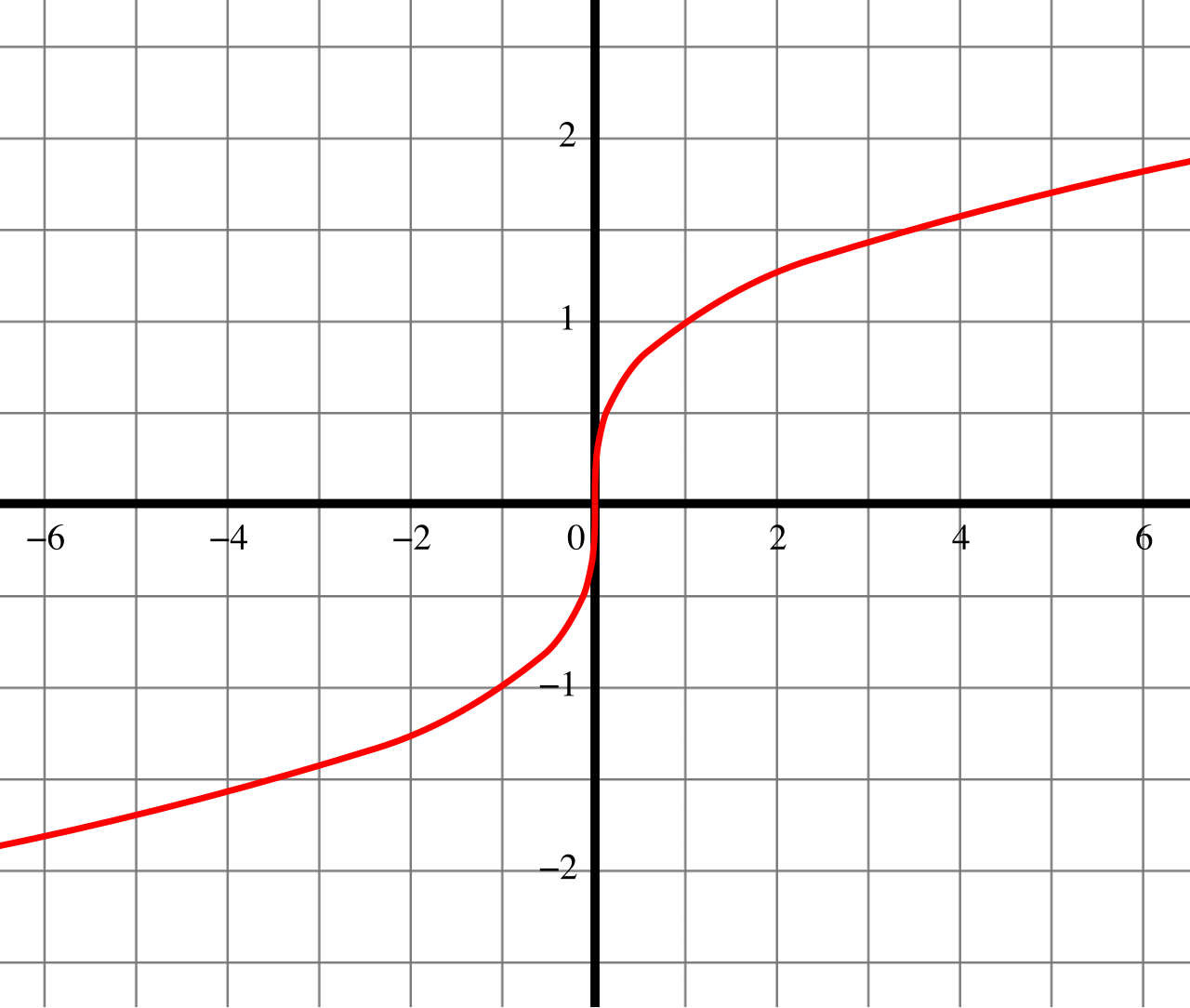
When algebraic manipulation divides out a common factor, the resulting graph accurately preserves the original domain restriction by displaying a removable discontinuity, or a "hole," rather than an intersection point.

Let us shift our focus to the inverse geometry of exponents: radicals. A radical equation contains at least one variable located inside the radicand of a radical expression. Note that if the radical simply has a number inside (like $\sqrt{3}x = 5$ ), it is a linear equation, not a radical one. Furthermore, keep in mind that the index of a standard square root symbol is implicitly two.

The Algorithm for Radicals

Solving a radical equation requires isolating a radical expression on one side of the equal sign. If you do not isolate the radical first, applying exponents will generate cross-terms that leave you tangled in an even worse algebraic mess than when you started.

Once isolated, the path is clear: Eliminating a radical expression of index $n$ requires raising both sides of the equation to the $n$ th power.

Reversibility and the Asymmetry of Powers

Here is where the magic—and the danger—of radical equations resides. Not all exponents behave the same way. The parity (evenness or oddness) of the index dictates the flow of algebraic truth.

Odd-index roots uniquely preserve the positive or negative sign of the original radicand. For example, $\sqrt[3]{8} = 2$ and $\sqrt[3]{-8} = -2$ . Because no sign information is lost, cubing or taking the cube root is a perfectly reversible street. Therefore, raising both sides of an equation to an odd integer power does not introduce extraneous solutions.

Unlike even roots, the graph of a cube root function maps smoothly into negative quadrants, illustrating how odd-index roots preserve sign information and maintain reversible operations.

Even powers, however, act like a mathematical black hole for negative signs. Raising both sides of an equation to an even integer power is a non-reversible operation. If I tell you that $x^2 = 25$ , you cannot definitively tell me if $x$ was originally $5$ or $-5$ . The sign information has been destroyed.

Because we lose information, raising both sides of an equation to an even integer power can introduce extraneous solutions.

The Principal Square Root

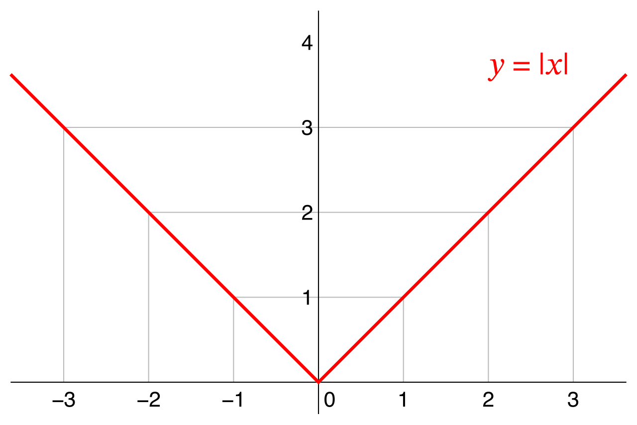
To deal with the ambiguity of even roots, mathematics relies on a strict definition. The principal square root of a non-negative real number evaluates to a non-negative value. This means $\sqrt{25}$ is strictly $5$ , not $\pm 5$ .

This leads to a deeply fundamental concept that you will teach repeatedly: The principal square root of the square of a real variable $x$ simplifies to the absolute value of $x$ .

$\sqrt{x^2} = |x|$

If $x = -3$ , then $\sqrt{(-3)^2} = \sqrt{9} = 3$ . This forces the output to be non-negative, perfectly matching the definition of the principal root.

The V-shaped graph of the absolute value function perfectly models the output of the principal square root of a squared variable, mathematically enforcing the rule of non-negativity.

Extraneous Solutions in Radical Equations

Because of this rigid non-negative output rule, algebraic manipulations can lead to absurdities. Suppose we have $\sqrt{x} = -4$ . The principal root cannot output a negative number, so there is no real solution. But watch what happens if a student blindly applies the algorithm:

Square both sides: $(\sqrt{x})^2 = (-4)^2$
Evaluate: $x = 16$

The student has found a solution! Or have they? An extraneous solution to a radical equation is an algebraically derived value that makes the original equation a false statement. If we plug $16$ back into the original equation, we get $\sqrt{16} = -4$ , which simplifies to $4 = -4$ . A blatantly false statement.

As a mathematics teacher, your ultimate goal is not just to teach students how to execute algorithms, but how to verify truth. The overarching narrative of rational and radical equations is that the algebraic machine is powerful, but blind. It will happily follow the rules of manipulation while walking straight off a logical cliff.

A common student error when solving radical equations is failing to substitute derived solutions back into the original equation to check for validity. Students often treat the final line of their algebra as the finish line of a race. You must reframe their thinking: arriving at $x = 16$ or $x = 2$ is merely the hypothesis. The proof only occurs when the value is subjected to the constraints of the original, unmanipulated equation.

Summary: The Dual Nature of Extraneous Solutions

When preparing for your exam—and your classroom—keep this distinction perfectly clear in your mind:

Equation Type	Operation that Causes Extraneous Solutions	What the Extraneous Solution Violates
Rational	Multiplying by an expression containing a variable (clearing the denominator).	The Domain. It attempts to force a division by zero.
Radical	Raising both sides to an even integer power.	The Truth Value. It attempts to make a positive principal root equal to a negative number, resulting in a false statement.

Teach your students to embrace the graphing calculator not as an answer key, but as an independent witness. Where the algebra lies by expanding domains and losing sign data, the graphs tell the truth through asymptotes, holes, and the strict absence of intersection points. By commanding both the abstract algebra and the visual geometry, you will guide your students safely through the traps of mathematical illusion.