Solving Systems of Equations

Not sure you’re ready?

Take the ~3-minute readiness diagnostic and see where you stand.

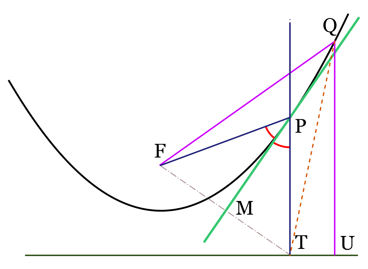
Imagine two objects moving through a two-dimensional plane—perhaps a commuter train following a straight track and a drone sweeping along a parabolic flight path. If we wish to know whether a collision is mathematically possible, we cannot analyze the train's route in isolation, nor the drone's. We must find a precise moment and location where both realities are simultaneously true. A system of equations is a set of two or more equations sharing the same variables, and solving it is the mathematical act of finding where distinct constraints overlap.

For the secondary mathematics teacher, systems of equations are the critical bridge between abstract algebraic manipulation and concrete geometric intuition. Your students will enter your classroom accustomed to solving for a single variable in a vacuum. Your task is to show them how multiple equations interact. To do this, we must formally define a solution to a system of two equations in two variables as an ordered pair that satisfies both equations simultaneously.

This guide will equip you with the deep conceptual framework required to master both linear and linear-quadratic systems for the Praxis (5165): Mathematics exam, ensuring you are prepared not just to calculate solutions, but to explain the why behind the mathematics.

Before we manipulate symbols, we must ground the algebra in geometry. Graphically representing a system of equations involves plotting each equation on the same coordinate plane. When we do this, the graphical solution to a system of equations corresponds to the exact points of intersection between the graphed functions.

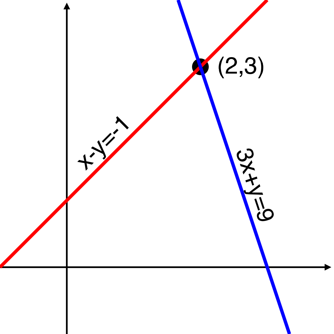
The graphical solution to an independent system of linear equations is the single coordinate point where the two lines intersect.

When dealing with linear systems, the behavior of these intersections is entirely dictated by the slopes and $y$ -intercepts of the lines. We can classify linear systems into three distinct categories based on their graphical and algebraic behavior:

System Classification	Definition	Graphical Representation	Algebraic Identifiers
Independent	An independent system of linear equations possesses exactly one unique solution.	Graphically, an independent system of two linear equations forms two lines intersecting at exactly one point.	Two linear equations exhibiting different slopes will always intersect at exactly one coordinate point. The $y$ -intercepts do not matter.
Dependent	A dependent system of linear equations possesses infinitely many valid solutions.	Graphically, a dependent system of two linear equations forms two coincident lines overlapping entirely.	Two linear equations sharing identical slopes and identical y-intercepts represent a dependent system. They are the exact same line.
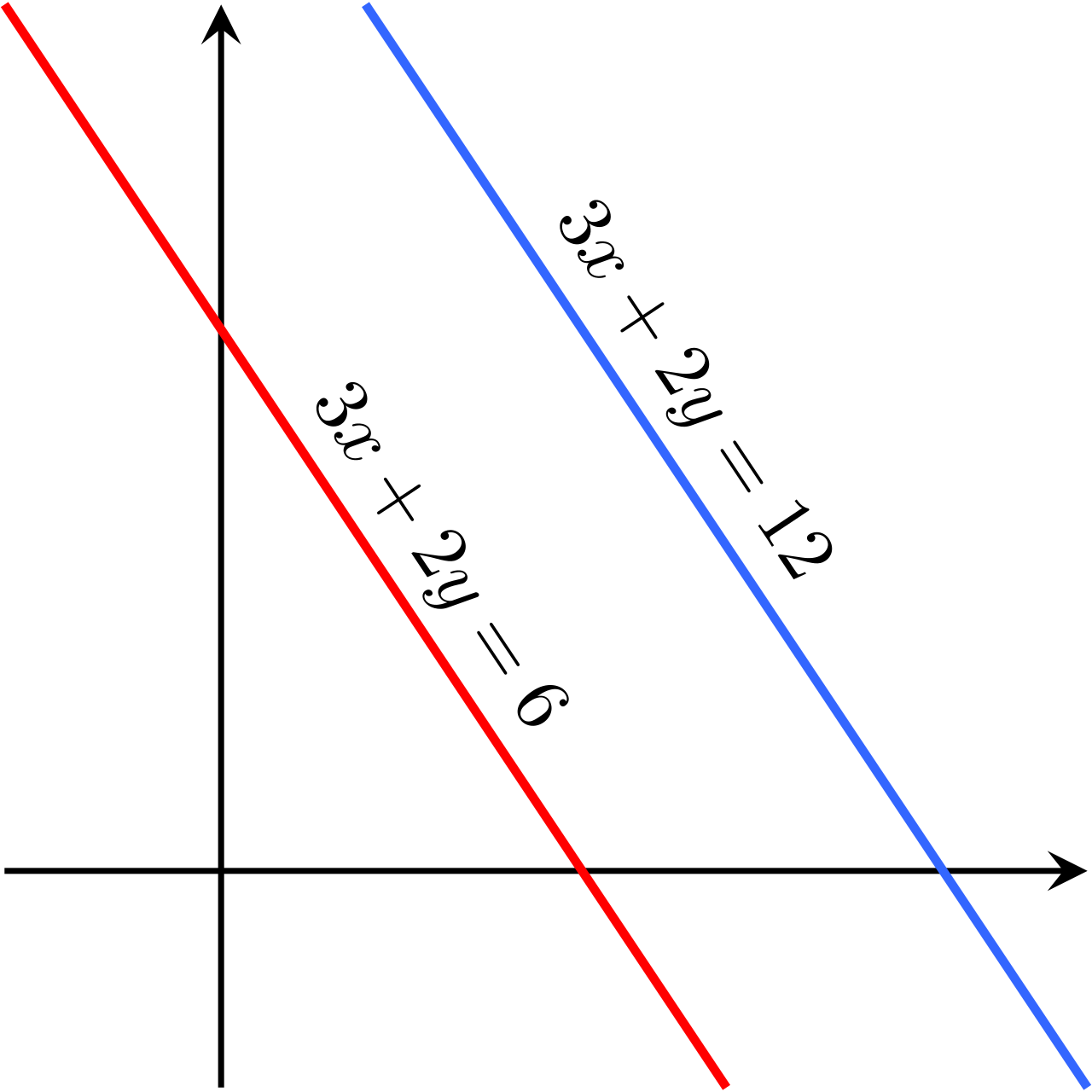
Inconsistent	An inconsistent system of linear equations contains zero valid solutions.	Graphically, an inconsistent system of two linear equations forms two parallel lines with no points of intersection.	Two linear equations sharing identical slopes and differing y-intercepts represent an inconsistent system.

Pedagogical Note on "Consistency" The term consistent simply means a truth exists. Therefore, a consistent system of linear equations is defined as a system possessing at least one valid solution. This broad umbrella encompasses both independent systems (one solution) and dependent systems (infinite solutions).

An inconsistent linear system forms parallel lines on a coordinate plane, proving geometrically that zero valid solutions can exist since the lines never intersect.

While graphing calculators are powerful diagnostic tools, analytic proofs require algebraic methods. There are two primary engines for solving linear systems algebraically: substitution and elimination. Both methods share the same underlying philosophy: reduce a two-variable problem into a one-variable problem.

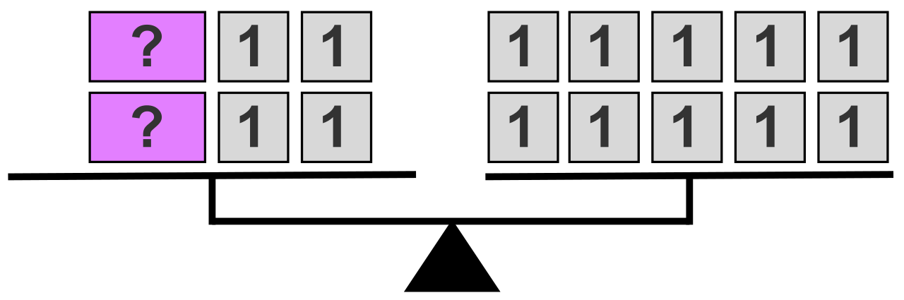
The balance scale is a classic pedagogical tool for visualizing the property of equality, reinforcing how manipulating equations during substitution and elimination maintains mathematical balance.

The Substitution Method

The substitution method is essentially mathematical embedding. The algebraic substitution method for solving a system begins by isolating one variable in one of the equations.

Once we have a statement like $y = 3x - 5$ , we have defined $y$ entirely in terms of $x$ . In the substitution method, the isolated variable expression is substituted into the second equation to create a single-variable equation. By replacing $y$ in the second equation with $(3x - 5)$ , the $y$ dimension collapses, leaving an equation purely in terms of $x$ that can be solved using fundamental arithmetic.

The Elimination Method

When an equation is written in standard form ( $Ax + By = C$ ), isolation can introduce messy fractions. Here, we use elimination. The algebraic elimination method involves adding or subtracting the given equations to eliminate a variable entirely.

This relies on the property of equality: if $A = B$ and $C = D$ , then $A + C = B + D$ . However, standard systems rarely align perfectly to cancel a variable out of the box. Therefore, in the elimination method, equations can be multiplied by non-zero constants to create opposite coefficients for a specific variable.

For example, if Equation 1 has a $2x$ and Equation 2 has a $3x$ , multiplying Equation 1 by $3$ and Equation 2 by $-2$ scales the equations so they feature $6x$ and $-6x$ , respectively. Adding them together annihilates the $x$ variable, paving the way to solve for $y$ .

The Praxis will test your ability to transcend straight lines. What happens when we introduce curvature?

Because a parabola curves back on itself, a system comprised of one linear equation and one quadratic equation can yield a maximum of two real coordinate solutions.

Just as with purely linear systems, the geometry provides an immediate, intuitive roadmap for the algebra. There are exactly three spatial scenarios for a line interacting with a parabola:

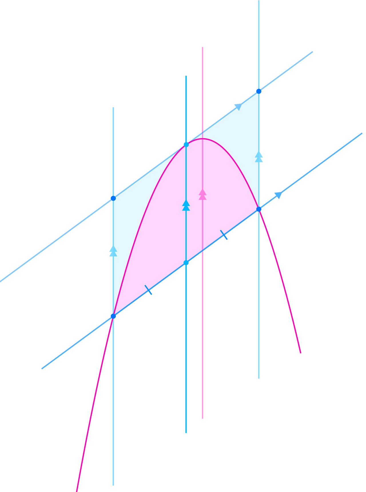
Two Intersections: A linear-quadratic system containing two real solutions graphically depicts a straight line intersecting a parabola at two distinct points (acting as a secant line).

When a linear-quadratic system possesses two real solutions, the linear equation acts as a secant line that intersects the parabola at two distinct coordinate points.

One Intersection: A system comprised of one linear equation and one quadratic equation can yield exactly one real coordinate solution. This highly precise scenario graphically depicts a straight line tangent to a parabola, merely grazing the curve at a single coordinate.

When a linear-quadratic system yields exactly one real solution, the line is perfectly tangent to the parabola, intersecting the curve at only a single coordinate.

No Intersections: A system comprised of one linear equation and one quadratic equation can yield zero real coordinate solutions. This graphically depicts a straight line that never intersects the parabola.

The Algebraic Engine for Linear-Quadratic Systems

To solve these systems, we rely heavily on substitution, as elimination is usually impossible due to mismatched degrees (you cannot add $x^2$ and $x$ to eliminate either).

Solving a linear-quadratic system algebraically typically requires isolating a variable in the linear equation first. (Attempting to isolate a variable in the quadratic equation often introduces $\pm$ square roots, which dramatically complicates the algebra).

Once isolated, substituting the isolated linear variable expression into the quadratic equation yields a new single-variable quadratic equation.

The Role of the Discriminant

Here is where many students—and teacher candidates—make a critical error. They look at the original parabola and calculate its discriminant ( $b^2 - 4ac$ ) to determine the number of solutions. This is entirely incorrect. The original parabola's discriminant only tells you if the parabola crosses the $x$ -axis. It tells you nothing about where it crosses the line.

Instead, the discriminant of the combined single-variable quadratic equation determines the total number of real solutions for the linear-quadratic system.

Once you substitute the linear expression into the quadratic and set the new equation to zero ( $Ax^2 + Bx + C = 0$ ), you evaluate $\Delta = B^2 - 4AC$ for this new equation:

A positive discriminant in the combined quadratic equation confirms that the linear-quadratic system possesses two distinct real solutions.
A discriminant of zero in the combined quadratic equation confirms that the linear-quadratic system possesses exactly one real solution.
A negative discriminant in the combined quadratic equation confirms that the linear-quadratic system possesses zero real solutions.

The Final Mile: Back-Substitution and Extraneous Roots

Finding the $x$ -values (or $y$ -values) using the combined quadratic equation is only half the battle. A coordinate is a pair. Each single-variable solution obtained in a linear-quadratic system must be substituted back into an original equation to determine the corresponding paired coordinate.

As a teacher, you must protect your students from a hidden trap during this final step. Mathematically, you can substitute the variable back into either the original linear equation or the original quadratic equation. However, substituting a solved variable back into the linear equation rather than the quadratic equation prevents the introduction of extraneous mathematical solutions.

Why does this matter? Consider the underlying mapping. A linear equation ( $y = mx + b$ ) represents a strictly one-to-one relationship; a specific $x$ yields exactly one $y$ . A quadratic relationship (such as $x = y^2 + 2$ ) is not one-to-one. If you solve the system and find $x = 6$ , plugging $6$ into $x = y^2 + 2$ yields $y^2 = 4$ , suggesting $y = 2$ and $y = -2$ . Suddenly, you have "created" a ghost coordinate that might not actually sit on your straight line!

By always back-substituting into the strict, single-path linear equation, you force the algebra to yield only the true, verifiable coordinate pair where both the line and the parabola exist in perfect agreement.