Quantitative Reasoning and Units

Not sure you’re ready?

Take the ~3-minute readiness diagnostic and see where you stand.

When a pure mathematician writes the number 7 on a chalkboard, it is a pristine, dimensionless abstraction. But in the physical sciences and in the applied mathematics you will teach, numbers rarely exist in a vacuum. Every physical measurement must include both a numerical magnitude and a specific unit. The moment we append a unit—7 meters, 7 seconds, 7 kilograms—we tether that abstraction to physical reality. Quantitative reasoning is the bridge between pure calculation and the physical world. For secondary mathematics students, mastering this bridge is what separates blind symbol manipulation from genuine mathematical modeling.

Pure mathematics explores abstract, dimensionless quantities such as the Mandelbrot set, contrasting with the unit-bound measurements of the applied physical sciences.

As an educator, you will frequently guide students through scenarios where the numbers alone are insufficient. Whether you are helping a student set the viewing window on a graphing calculator, grading a physics-crossover problem, or showing them why a carpet installation estimate is wrong, units and scales are the fundamental vocabulary of applied mathematics.

Before we manipulate data algebraically, we must represent it visually. The translation from physical reality to a two-dimensional graph requires strict geometric rules.

Origins and Scales

When graphing, the origin of a graph represents the zero value for both the independent and dependent variables. It is the absolute reference point from which all physical geometry on the Cartesian plane radiates.

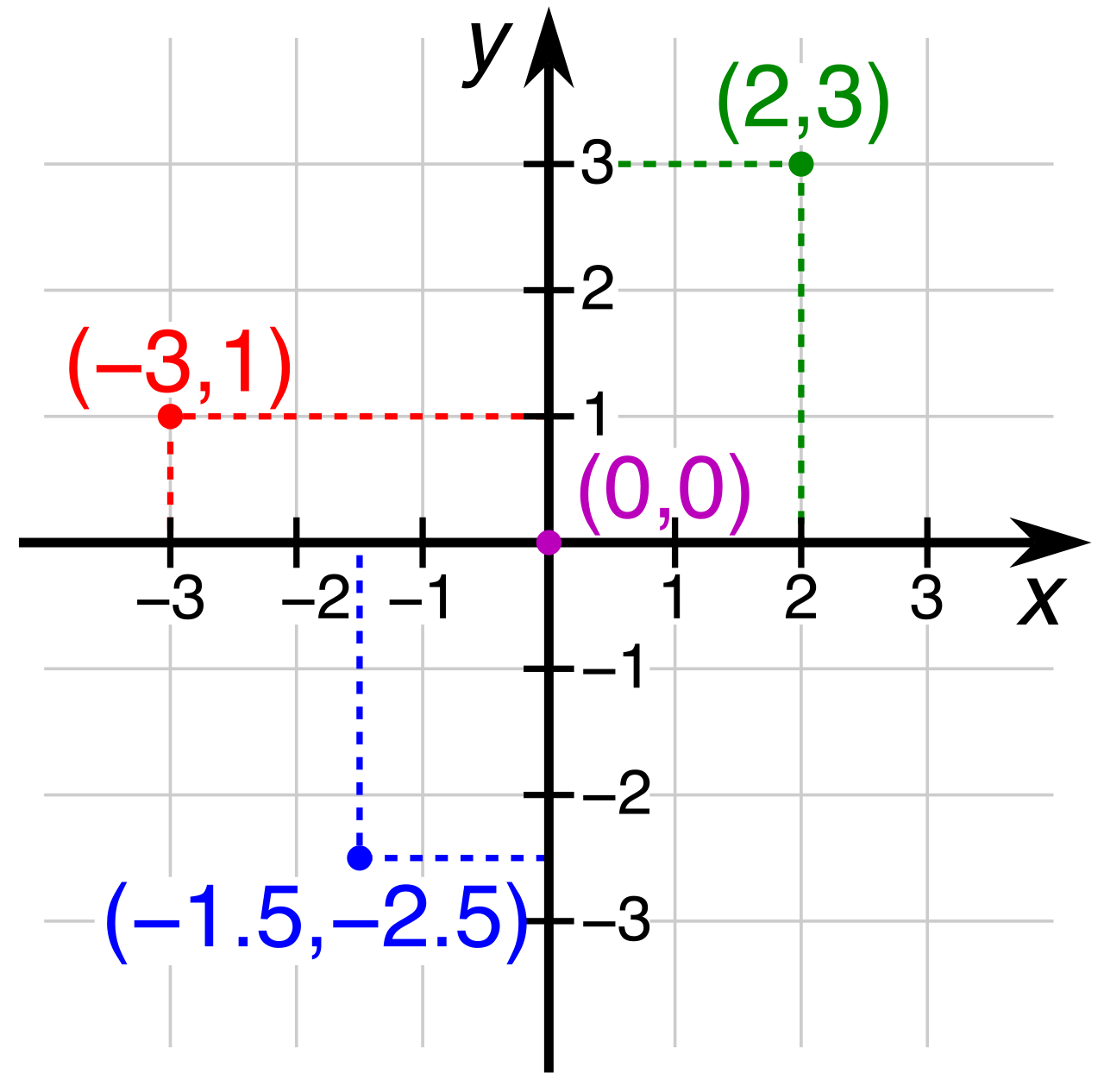
In the Cartesian coordinate system, the origin (0,0) serves as the absolute zero-reference point for both independent and dependent variables.

However, raw data rarely fits neatly onto default grid lines. The scale on a graph determines the mathematical relationship between the graphical units and the real-world quantities. When you or your students are confronted with a scatterplot or a functional model, selecting an appropriate graph scale requires finding a constant interval that accommodates the minimum and maximum data values. If a student is tracking a projectile that reaches a maximum height of 450 feet over 12 seconds, setting the graphing calculator window requires scaling the horizontal $x$ -axis (time) in 1- or 2-second constant intervals, while the vertical $y$ -axis (height) might require constant intervals of 50 feet.

Axis Breaks and Visual Distortion

Sometimes, the data clusters far away from the origin. In these cases, we might use a graph break (often drawn as a squiggle or a double slash on the axis). An axis break in a graph indicates a skipped range of numerical values.

While this saves space, you must caution your students: an axis break can visually distort the proportional relationship between the graphed data points. If a bar chart starts at 90 instead of 0, a value of 95 will look twice as large as a value of 91, even though it is proportionally only marginally larger. Teaching students to recognize this distortion is a critical component of quantitative literacy.

Dimensionality in Calculus Prep: Slope and Area

When we graph physical quantities, the geometric properties of the graph hold deep physical meaning. Look at the units; they tell the story of the mathematics.

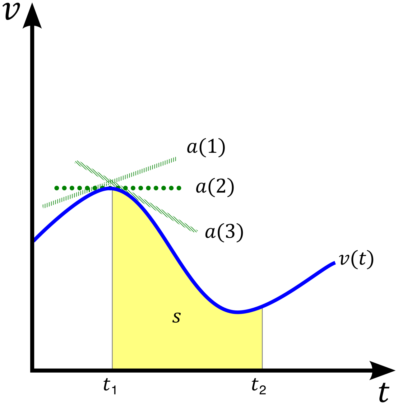
The units of the slope of a graphed line are the units of the vertical axis divided by the units of the horizontal axis.
- Example: If the $y$ -axis is distance (meters) and the $x$ -axis is time (seconds), the slope units are meters/second.
The units of the area under a curve are the units of the vertical axis multiplied by the units of the horizontal axis.
- Example: If the $y$ -axis is velocity (meters/second) and the $x$ -axis is time (seconds), the area units are $(\text{meters/second}) \times \text{seconds} = \text{meters}$ .

Teacher's Note: Highlighting unit relationships in slope and area provides secondary students with an intuitive preview of derivatives (rates of change) and integrals (accumulation), long before they encounter formal calculus.

In a velocity versus time graph, the geometric properties carry specific physical units: the slope represents acceleration, and the area under the curve represents accumulated displacement.

Because measurements map to the real world, they are inherently limited by the tools we use. We must distinguish between how careful we are and how correct we are.

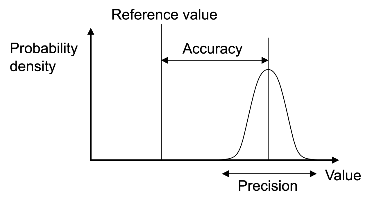
Measurement precision refers to the level of detail or the smallest incremental value of the measuring instrument. A ruler with millimeter markings is more precise than a yardstick with only inch markings.
Measurement accuracy refers to how closely a measured value matches the true or accepted physical value. You can have a highly precise instrument (like a digital scale reading to 0.001 grams) that is improperly calibrated, yielding very precise but highly inaccurate results.

Accuracy describes how closely a measurement aligns with the true value, whereas precision describes the level of detail and reproducibility of the measuring instrument.

Significant Figures

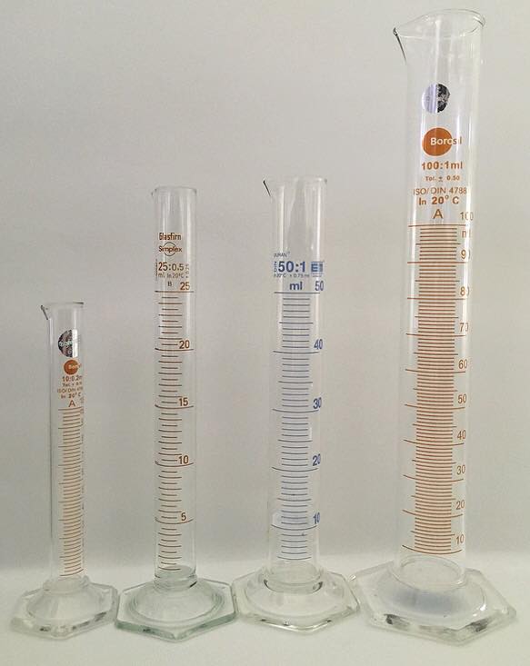
To communicate the precision of our tools mathematically, we use significant figures. Significant figures represent all the certain digits in a measurement plus one estimated digit. If a liquid aligns between the 42 mL and 43 mL marks on a graduated cylinder, a student might record 42.4 mL. The '4' and '2' are certain; the '.4' is the one estimated digit. All three are significant.

When reading a graduated cylinder, the recorded measurement must include all certain digits derived from the scale markings plus one final estimated digit.

When manipulating these measurements algebraically, the precision of our output cannot exceed the precision of our input. We are bound by two distinct rules:

Addition and Subtraction Rule: In addition of measurements, the final sum must be rounded to the same decimal place as the least precise measurement. (Example: $12.1 \text{ cm} + 3.05 \text{ cm} = 15.15 \text{ cm}$ , which rounds to $15.2 \text{ cm}$ because the first measurement only goes to the tenths place.)

Multiplication and Division Rule: In multiplication of measurements, the final product must have the same number of significant figures as the measurement with the fewest significant figures. (Example: $4.56 \text{ m} \times 1.4 \text{ m} = 6.384 \text{ m}^2$ , which rounds to $6.4 \text{ m}^2$ because 1.4 only has two significant figures.)

One of the most powerful tools you can give a mathematics student is the realization that units obey the exact same algebraic laws as variables like $x$ or $y$ .

Dimensional analysis is a problem-solving method that uses the physical units of quantities to guide mathematical calculations. In dimensional analysis, physical units are algebraically manipulated exactly like variables. If you have $x \cdot \frac{y}{x}$ , the $x$ 's cancel out. Similarly, physical units can be algebraically canceled out when the same unit appears in both the numerator and the denominator of a product.

Arithmetic with Units

This algebraic behavior explains our rules for combining quantities:

Adding physical quantities mathematically requires all the quantities to possess identical measurement units. You can add $3x + 2x = 5x$ , and you can add $3 \text{ kg} + 2 \text{ kg} = 5 \text{ kg}$ . You cannot add $3 \text{ kg} + 2 \text{ meters}$ any more than you can simplify $3x + 2y$ .
Subtracting physical quantities mathematically requires all the quantities to possess identical measurement units.

Fundamental vs. Derived Units

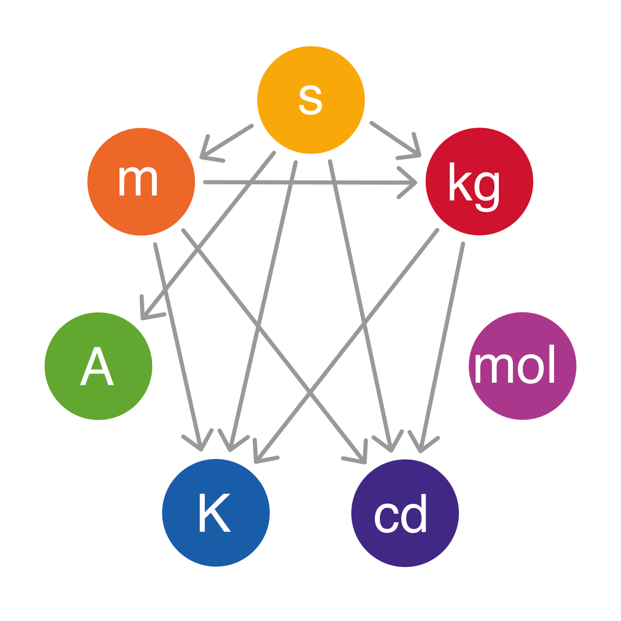
While we add identical units, we can multiply and divide different units to forge new concepts. Derived units are created by multiplying or dividing fundamental measurement units.

Speed is a derived unit created by dividing a distance measurement by a time measurement. (e.g., miles per hour).
Density is a derived unit created by dividing a mass measurement by a volume measurement. (e.g., grams per cubic centimeter).

The International System of Units (SI) relies on seven base units, from which all other derived units (such as speed or density) are created via multiplication or division.

Often, we have a measurement in one unit, but we need it in another. This is where conversion factors come into play. A conversion factor is a mathematical ratio expressing the exact equivalence between two different units of measurement.

Here is the beautiful trick of conversion: A unit conversion factor ratio is always mathematically equal to the dimensionless number one.

Because $1 \text{ hour} $is exactly the same amount of time as \$ 3600 \text{ seconds} $, the ratio$ \frac{3600 \text{ s}}{1 \text{ hr}} $evaluates to$ 1 $. **Multiplying a physical quantity by a valid unit conversion factor does not change the actual physical amount.** It merely changes the numerical magnitude and the specific unit used to describe that amount. It is the physical equivalent of finding a [common denominator](https://en.wikipedia.org/wiki/Lowest_common_denominator) by multiplying a [fraction](https://en.wikipedia.org/wiki/Fraction_%28mathematics%29) by$ \frac{3}{3}$.

Essential Equivalence Facts

For the Praxis exam, you must have immediate fluency with fundamental conversion equivalencies. Consider this your mathematical toolbox:

Metric Equivalencies	Customary & Mixed Equivalencies
One kilometer is equal to exactly 1000 meters.	One mile is equal to exactly 5280 feet.
One meter is equal to exactly 100 centimeters.	One inch is defined as exactly 2.54 centimeters.
	One kilogram is approximately equal to 2.205 pounds.
	One gallon is equal to exactly 4 quarts.
	One hour is equal to exactly 3600 seconds.

Note: Pay attention to the definitions. The relationship between inches and centimeters is mathematically exact by international agreement, whereas the relationship between kilograms and pounds is an approximation depending on gravitational force.

The Area and Volume Trap

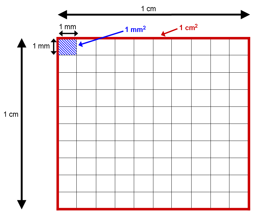
There is a classic cognitive trap that will catch your students, and you must be prepared to help them navigate it. If a student knows that $1 \text{ meter} = 100 \text{ centimeters} $, they will frequently guess that \$ 1 \text{ square meter} = 100 \text{ square centimeters}$.

Let us use dimensional analysis to show why this is false. To find an area, we multiply length by width. If we want to convert $1 \text{ m}^2 $into$ \text{cm}^2 $, we must multiply by our conversion factor$ \left( \frac{100 \text{ cm}}{1 \text{ m}} \right) $*twice* to cancel out$ m \cdot m$.

$1 \text{ m}^2 \times \left( \frac{100 \text{ cm}}{1 \text{ m}} \right) \times \left( \frac{100 \text{ cm}}{1 \text{ m}} \right) = 10,000 \text{ cm}^2$

Converting square units requires squaring the linear conversion factor. For instance, because 1 cm equals 10 mm, 1 square centimeter contains 100 square millimeters.

Converting square measurement units requires squaring the standard linear conversion factor.
Converting cubic measurement units requires cubing the standard linear conversion factor. (e.g., $1 \text{ m}^3 = 100^3 \text{ cm}^3 = 1,000,000 \text{ cm}^3$).

When you stand in front of a classroom, your goal is to help students see that mathematics is not a set of arbitrary rules, but the language nature is written in. By interpreting scales and origins thoughtfully, respecting the rules of accuracy and precision, and treating units as algebraic entities through dimensional analysis, you empower students to navigate the real world quantitatively. Remember the units, and the math will guide you home.