Sampling and Study Design
Not sure you’re ready?
Take the ~3-minute readiness diagnostic and see where you stand.
A chef does not need to consume an entire vat of soup to know if it requires more salt. By stirring the pot thoroughly and tasting a single spoonful, the chef grasps the flavor of the whole. As a mathematics educator, you face a similar reality: you cannot constantly assess every student on every conceivable mathematical concept without paralyzing your classroom. Instead, you extract samples of their knowledge. When we step back from the classroom into the broader realm of statistics, this fundamental act of sampling—pulling a fragment from the whole to understand the universe it came from—forms the bedrock of empirical truth. The transition from scattered data points to justified, generalized conclusions requires a rigorous architecture. Without careful study design, data is just noise masquerading as evidence.
To make sense of a population, we first must decide how we interact with it. The defining distinction in study design lies in whether we merely watch the universe or whether we reach out and manipulate it.
An observational study records data on individuals without attempting to influence the responses. It measures variables of interest without assigning treatments to subjects. If you want to know whether high schoolers who take calculus sleep fewer hours than those who do not, you simply ask them. A sample survey is a specific type of observational study designed to collect data from a subset of a population. Conversely, a census is a study attempting to collect data from every individual in the entire population.
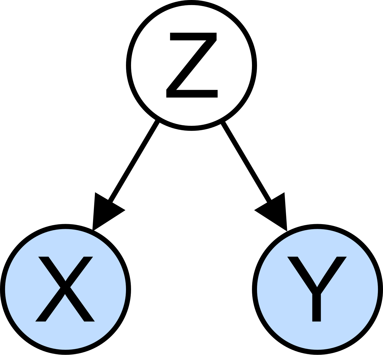
Can surveying students about calculus and sleep prove that the rigorous math is causing the sleep deprivation? Absolutely not. An observational study cannot definitively establish a cause-and-effect relationship. The culprit preventing this causal leap is the confounding variable—a third variable related to both the explanatory variable and the response variable. Perhaps students who take calculus are also highly motivated high-achievers juggling three varsity sports and a part-time job. This internal drive creates false statistical associations between the explanatory variable (taking calculus) and the response variable (lack of sleep).
To isolate the truth, we must switch from observation to intervention. An experiment deliberately imposes a treatment on individuals to measure corresponding responses. Only a well-designed experiment can establish a cause-and-effect relationship between variables because it is designed to strip away the noise of confounding factors.
In statistics, we differentiate between the universe and our localized slice of it. A parameter is a fixed numerical characteristic describing an entire population (like the true average GPA of all high school students in the United States). A statistic is a numerical characteristic calculated from a sample dataset. We use statistics to guess at parameters.
For our guesses to be valid, our sampling method must be immaculate. Random sampling involves selecting members from a population using a chance process. This is non-negotiable if we wish to look outward; random sampling allows researchers to generalize study results to the broader population.
Methods of Random Sampling
-
Simple Random Sample (SRS): The gold standard. A simple random sample gives every individual in the population an equal chance of being selected, and crucially, it gives every possible sample of the same size an equal chance of being selected.
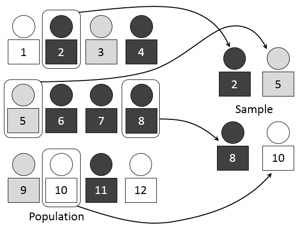
In a simple random sample, every individual and every possible sample of the specified size has an equal probability of selection. Source: Simple random sampling by Dan Kernler, CC BY-SA 4.0. -
Stratified Random Sampling: Suppose you want to survey students on a proposed block schedule. Freshmen and seniors likely have vastly different opinions. Stratified random sampling divides the population into distinct homogeneous groups (the grade levels) before selecting a simple random sample from each group.
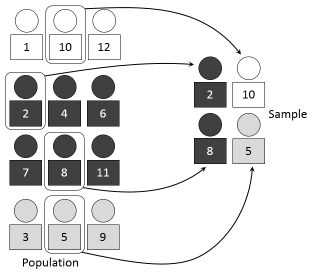
Stratified sampling divides the population into homogeneous subgroups (strata) before drawing a random sample from within each group. Source: Stratified sampling by Dan Kernler, CC BY-SA 4.0. -
Cluster Sampling: Imagine your school’s homerooms are all mixed-ability, mixed-grade microcosms. Cluster sampling divides the population into heterogeneous groups and conducts a census on randomly selected groups. You choose three homerooms at random and survey every student inside them.
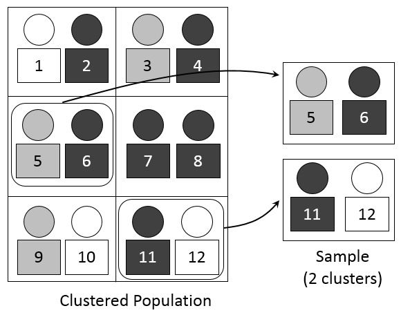
Cluster sampling groups the population into mixed subgroups, randomly selects entire subgroups, and surveys every individual within them. Source: Cluster sampling by Dan Kernler, CC BY-SA 4.0. -
Systematic Random Sampling: This selects every kth individual from a population list after a random starting point. If k=10, you pick a random starting student between 1 and 10, then select every 10th student on the roster thereafter.
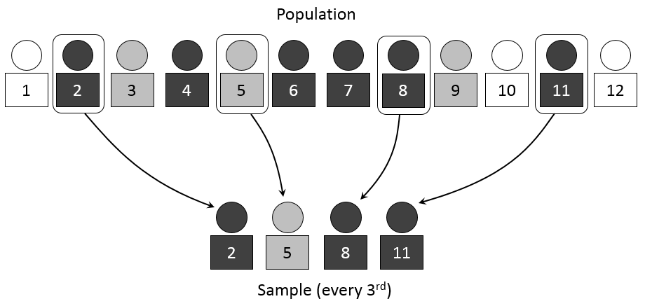
Systematic sampling selects every kth member of a population from an ordered list after establishing a random starting point. Source: Systematic sampling by Dan Kernler, CC BY-SA 4.0.
When Sampling Goes Awry
When we abandon chance, we invite statistical bias, which is the systematic overestimation or underestimation of a population parameter. By contrast, an unbiased estimator has a sampling distribution with a mean equal to the true value of the population parameter. Flawed sampling ruins this elegance:
-
Convenience sampling selects individuals who are easiest to reach for the researcher (e.g., surveying the students in your front row). Convenience sampling frequently produces biased data unrepresentative of the population.
-
Voluntary response bias occurs when individuals self-select to participate in a survey. Only those with fierce opinions bother to respond.
-
Undercoverage occurs when some members of the population are inadequately represented in the sampling frame (e.g., conducting a phone survey during school hours excludes most teenagers).
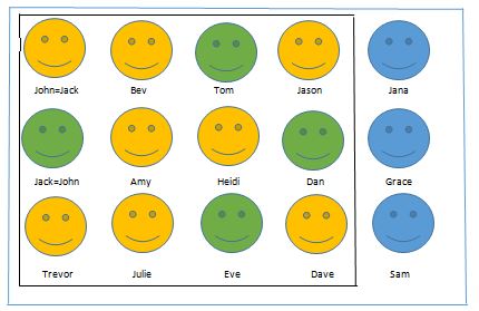
Undercoverage occurs when the sample frame fails to accurately capture the entire target population, leaving some members with no chance of selection. Source: CoverageError by The Jedi Math Squirrel, CC BY-SA 4.0. -
Nonresponse bias occurs when selected individuals cannot be contacted or refuse to participate in a study.
-
Response bias occurs when participants provide incorrect or untruthful answers to survey questions, perhaps due to poorly worded questions or social pressure.
While random sampling determines who is in the study, random assignment dictates what happens to them once they are there. These two concepts are frequently conflated, yet their roles are entirely distinct. Random assignment involves distributing experimental units to treatment groups using a chance process.
Why rely on chance? Because random assignment helps ensure treatment groups are roughly equivalent before an experiment begins. By scattering the over-achievers, the exhausted, and the brilliant evenly across all groups, random assignment minimizes the effects of unknown confounding variables across treatment groups. Consequently, random assignment allows researchers to make causal conclusions about the effect of a treatment.
Key Features of a Valid Experiment
The Placebo and the Control: How do you know a new math tutoring software works? You need a control group, a baseline group receiving no treatment or a standard neutral treatment. Often in human trials, the control group receives a placebo, a fake treatment given to a control group to mimic the experience of the active treatment. This accounts for the placebo effect, which occurs when subjects show a response to a dummy treatment due to the expectation of receiving an active treatment.
Blinding: If a student knows they are receiving the "inferior" standard curriculum, their morale might drop, skewing the data. In a single-blind experiment, subjects do not know which specific treatment is being administered to them. If the teacher grading the assessments also knows who received the special software, they might unconsciously grade them more favorably. In a double-blind experiment, neither the subjects nor the interacting researchers know the treatment assignments.
Structuring the Groups
How we deploy random assignment dictates the experimental design:
- Completely Randomized Design: The simplest method. It randomly assigns all experimental units among all available treatments.
- Randomized Block Design: If we suspect that prior math ability strongly affects a student's response to the new software, we first block them by past grades. A randomized block design groups similar experimental units together before randomly assigning treatments within each group.
- Matched Pairs Design: A highly precise block design. A matched pairs design groups subjects into sets of two similar individuals to receive different treatments. Alternatively, a matched pairs design can involve a single subject receiving both treatments in a randomized order (e.g., taking a pre-test with a standard calculator, then a post-test with a graphing calculator, with half the class doing the reverse order).
Once the data is gathered, the mathematical heavy lifting begins. We use sample statistics to estimate population parameters.
- A sample proportion (p^) serves as a point estimate for an unknown population proportion (p).
- A sample mean (xˉ) serves as a point estimate for an unknown population mean (μ).
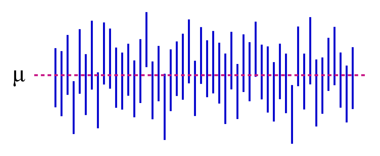
But a point estimate is rarely perfectly accurate. To capture reality, we construct a confidence interval, which provides a range of plausible values for an unknown population parameter. A confidence interval is calculated by adding and subtracting the margin of error from the sample point estimate.
The margin of error describes the maximum expected difference between a sample point estimate and the true population parameter. It is the mathematical buffer we create to account for sampling variability.
The Mathematics of the Margin of Error
The margin of error calculation requires multiplying a critical value by the standard error of the statistic.
Margin of Error=(Critical Value)×(Standard Error)
The standard error estimates the standard deviation of the sampling distribution of a statistic.
- The standard error of a sample proportion is the square root of the product of the sample proportion and its complement divided by the sample size: np^(1−p^).
- The standard error of a sample mean is the sample standard deviation divided by the square root of the sample size: ns.
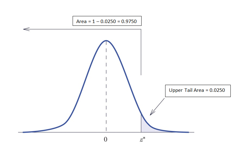
The critical value is a Z-score (for proportions or large sample means) derived from the standard normal distribution, determined entirely by how confident we wish to be.
- The critical z-score for a 90 percent confidence level using a standard normal distribution is approximately 1.645.
- The critical z-score for a 95 percent confidence level using a standard normal distribution is approximately 1.96.
- The critical z-score for a 99 percent confidence level using a standard normal distribution is approximately 2.576.
The Push and Pull of Sample Size and Confidence
Consider the dynamics of this formula. The denominator of the standard error contains n, meaning the sample size n is inversely proportional to the standard error. Therefore, increasing the sample size generally decreases the margin of error. Fundamentally, increasing the sample size reduces the variability of the sampling distribution; a larger sample provides a sharper, more focused picture of the truth.
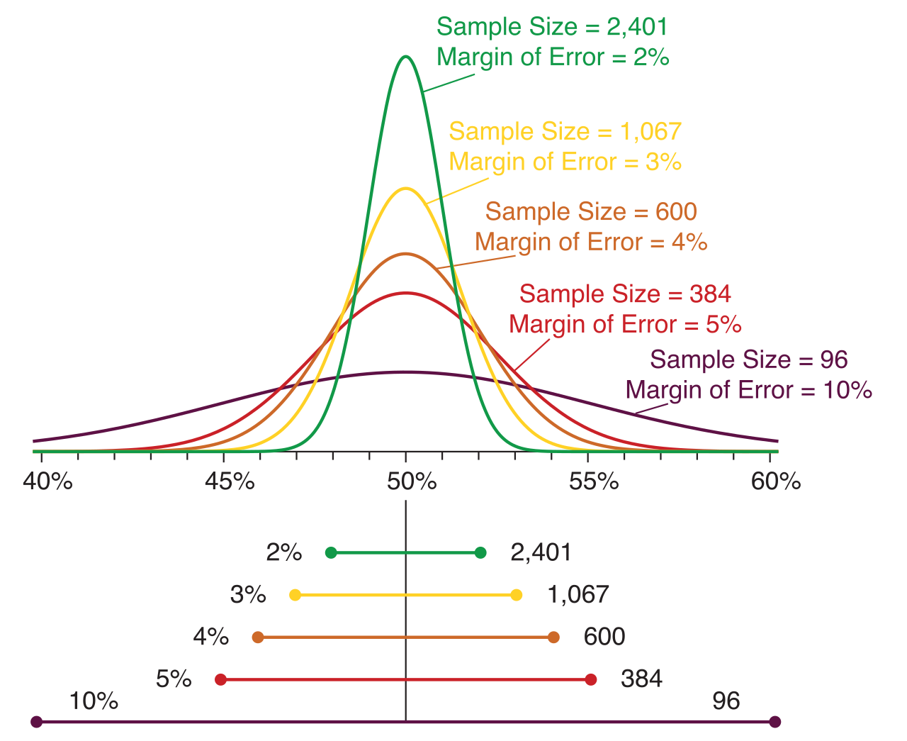
However, confidence comes at a cost. If you wish to be more certain that your interval captures the true parameter, you must cast a wider net. You shift your critical value from 1.96 up to 2.576. Thus, increasing the required confidence level increases the resulting margin of error.
When you teach your future students to design an experiment or survey, you are teaching them how to filter the chaotic signal of reality. Recognizing biases, ensuring proper randomization, and understanding the elegant mechanics of confidence intervals are not merely abstract academic hoops. They are the analytical lenses through which educated citizens—and exceptional mathematicians—discern truth from coincidence.