Population Dynamics

Not sure you’re ready?

Take the ~3-minute readiness diagnostic and see where you stand.

A single bacterium, reproducing by binary fission every twenty minutes, possesses the mathematical potential to eventually form a mass of cells heavier than the Earth itself. We know, instinctively, that this never happens. The physical world intervenes. Understanding exactly how and why the environment restrains life is the core of demography, the statistical study of population changes over time. As a biology educator, your task is to show students that population dynamics are not just a collection of abstract graphs, but a reflection of the brutal, beautiful calculus of survival.

Whether you are tracking the explosive spread of an invasive weed or managing a recovering herd of local deer, every ecological scenario requires analyzing the population growth rate, defined strictly as the change in the number of individuals in a population over a specific time period.

To understand how populations function, we must first model them under ideal conditions, and then apply the friction of reality.

The Exponential Growth Model

The exponential growth model assumes resources are unlimited in an environment. Imagine a newly established colony of bacteria in a vast, nutrient-rich Petri dish. Without space or food constraints, the population accelerates continuously, which results in a J-shaped population growth curve over time.

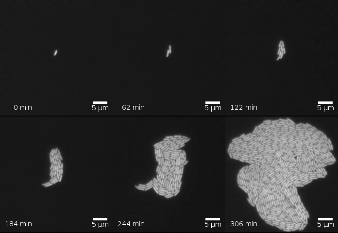
Under optimal conditions with unlimited resources, bacterial colonies exhibit exponential growth, resulting in a classic J-shaped population curve.

Mathematically, this is expressed elegantly:

Equation for Exponential Population Growth: dN/dt = rmax * N

In this exponential growth equation, the intrinsic rate of increase ( $r_{max}$ ) is multiplied by the current population size ( $N$ ). But what is this intrinsic rate? Simply put, the intrinsic rate of increase represents the per capita birth rate minus the per capita death rate. As long as births exceed deaths even slightly, and resources remain infinite, the larger the population gets, the faster it grows.

The Logistic Growth Model

But the Earth is finite. A forest has a limited canopy; a pond has a limited amount of dissolved oxygen. The logistic growth model accounts for resource limitations in an environment.

Because environments cap growth, logistic population growth results in an S-shaped curve over time. The ceiling of this curve is the carrying capacity, which is the maximum population size that a specific environment can sustain indefinitely.

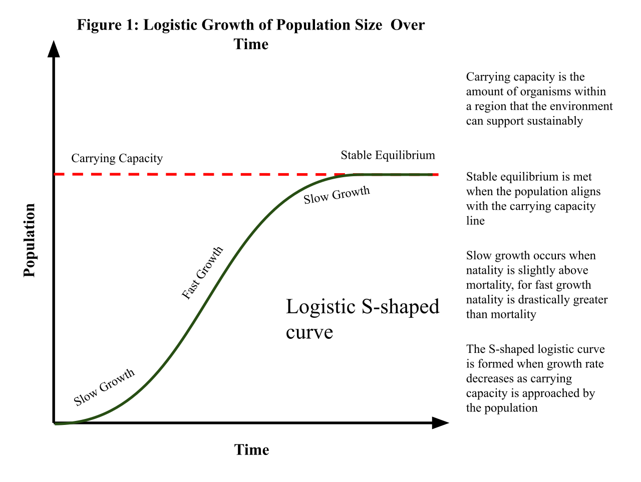
The logistic growth model demonstrates how a population's growth rate decelerates and levels off as the number of individuals approaches the environment's carrying capacity (K).

Equation for Logistic Population Growth: dN/dt = rmax * N * ((K-N)/K)

In all population growth equations, carrying capacity is represented by the variable K.

Notice the brilliant addition to our previous equation: the term (K-N)/K. This term represents the fraction of carrying capacity still available for population growth.

Imagine a theater with 100 seats ( $K = 100$ ).
If only 2 people are inside ( $N = 2$ ), the available space is $(100 - 2) / 100 = 0.98$ . The population grows at 98% of its maximum potential.
If 99 seats are filled ( $N = 99$ ), the available space is $1 / 100 = 0.01$ .

Through this mathematical mechanism, the logistic growth model dictates that the population growth rate slows as the population size approaches the carrying capacity. If a sudden influx of individuals occurs, causing the population size to exceed the environmental carrying capacity, the population experiences negative growth until it falls back below the sustainable threshold.

The forces that dictate carrying capacity and constrain the growth, abundance, or distribution of a population are known collectively as limiting factors. These are broadly categorized by how they respond to population density.

Density-Dependent Limiting Factors

Density-dependent limiting factors are usually biotic components of the ecosystem. Crucially, the impact of density-dependent limiting factors increases as population density increases. As organisms crowd together, life gets inherently more difficult.

Common density-dependent constraints include:

Intraspecific competition: As a population grows, individuals of the same species must compete harder for diminishing resources like food, water, and nesting sites.
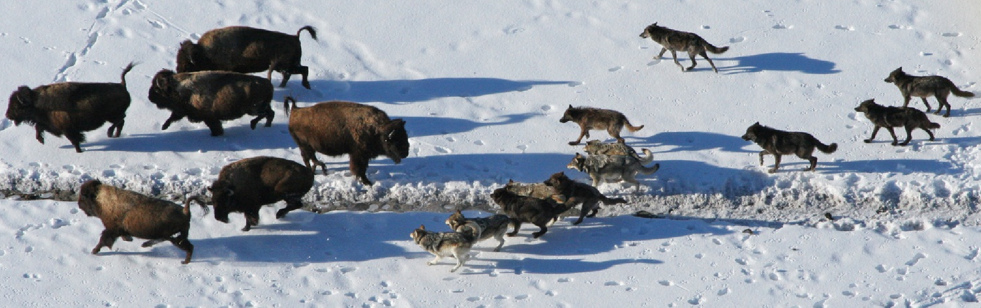
Predation: A dense population is an easy target. Predation acts as a density-dependent limiting factor because predators will preferentially hunt abundant prey.
Disease: Infectious diseases spread more rapidly in dense populations. Pathogen transmission acts as a density-dependent limiting factor—something we experience intuitively when a cold sweeps through a crowded high school but spares isolated rural communities.
Waste: The accumulation of toxic waste products in a habitat is a density-dependent limiting factor. Yeast in a wine vat, for example, will eventually die from the concentrated alcohol they produce.

Predation acts as a powerful density-dependent limiting factor, as predators—like these wolves working cooperatively to hunt bison—often find it easier to locate and capture prey when prey populations are dense.

Density-Independent Limiting Factors

Conversely, density-independent limiting factors are usually abiotic components of the ecosystem. The impact of density-independent limiting factors is constant regardless of population density.

A hurricane does not care if there are ten birds in a tree or ten thousand; the destructive force is identical. Examples include:

Severe weather events (e.g., floods, deep freezes).
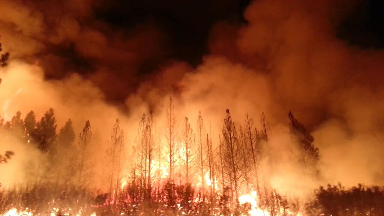
Natural disasters such as wildfires.
Environmental pollutants, such as an oil spill in a marine bay.

Density-independent limiting factors, such as severe wildfires, drastically reduce local population sizes indiscriminately, regardless of how crowded or sparse the population was prior to the event.

The Exception to the Crowding Rule: The Allee Effect

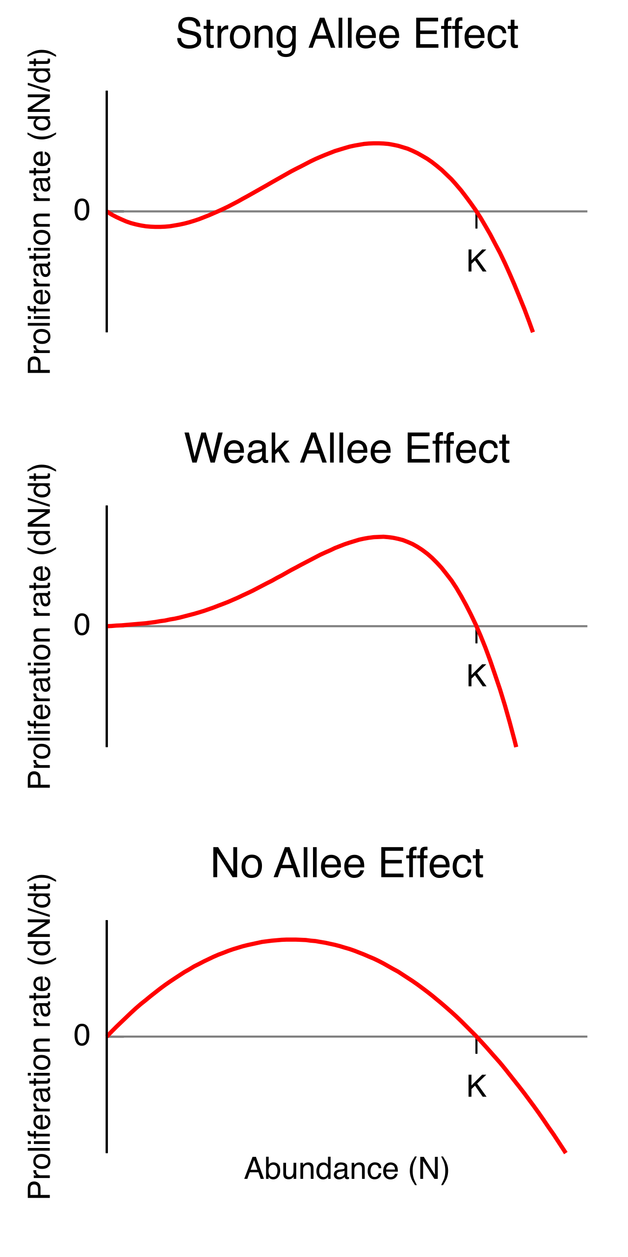
While high density usually suppresses growth, extremely low density brings its own perils. The Allee effect occurs when a population's per capita growth rate decreases as population density drops below a critical threshold. Think of a severely depleted population of whales scattered across an ocean. Even with abundant food, if they cannot physically locate each other to mate, the population's growth stalls.

The Allee effect illustrates that at extremely low population densities, the per capita growth rate can decline rather than increase, potentially driving a severely depleted population toward extinction.

Organisms have finite energy. They can either use it to produce a massive amount of "cheap" offspring, or a tiny amount of "expensive" offspring. The r/K selection theory relates parental reproductive strategies to environmental fluctuations.

Feature	r-strategists (The Lottery)	K-strategists (The Investment)
Habitat Stability	r-selected species thrive in environmentally unstable habitats.	K-selected species thrive in environmentally stable habitats.
Offspring Quantity	Produce a large number of offspring during each reproductive event.	Produce a small number of relatively large offspring.
Parental Care	Offspring receive little to no parental care.	Offspring receive significant parental care.
Maturation & Size	Typically reach sexual maturity early in life and possess small body sizes.	Typically reach sexual maturity late in life and possess large body sizes.
Population Dynamics	Prone to boom-and-bust cycles.	K-selected populations tend to remain close to the environmental carrying capacity.
Classic Examples	Dandelions (plants); marine invertebrates like oysters (animals).	Elephants and humans.

Marine invertebrates like oysters are highly r-selected species. An oyster might release millions of eggs into the turbulent ocean—buying millions of "lottery tickets"—knowing virtually all will perish. Conversely, elephants are an example of a K-selected animal species, investing years into raising a single calf to ensure its survival in a highly competitive, stable savanna.

Highly r-selected species, such as dandelions relying on wind-driven seed dispersal, invest minimal energy into each individual offspring, expecting the vast majority to perish.

To track these differing life strategies mathematically, ecologists rely on specific demographic tools.

When researchers study a population, they often follow a cohort, which is a group of individuals of the same species born at roughly the same time (much like tracking a high school graduating class). They track these cohorts using life tables, which summarize the survival and reproductive rates of individuals in specific age groups within a population. A key metric in these tables is fecundity, defined as the potential reproductive capacity of an individual or population.

Survivorship Curves

Plotting the data from life tables reveals three distinct survivorship curves, which visually map directly onto our r/K selection theory.

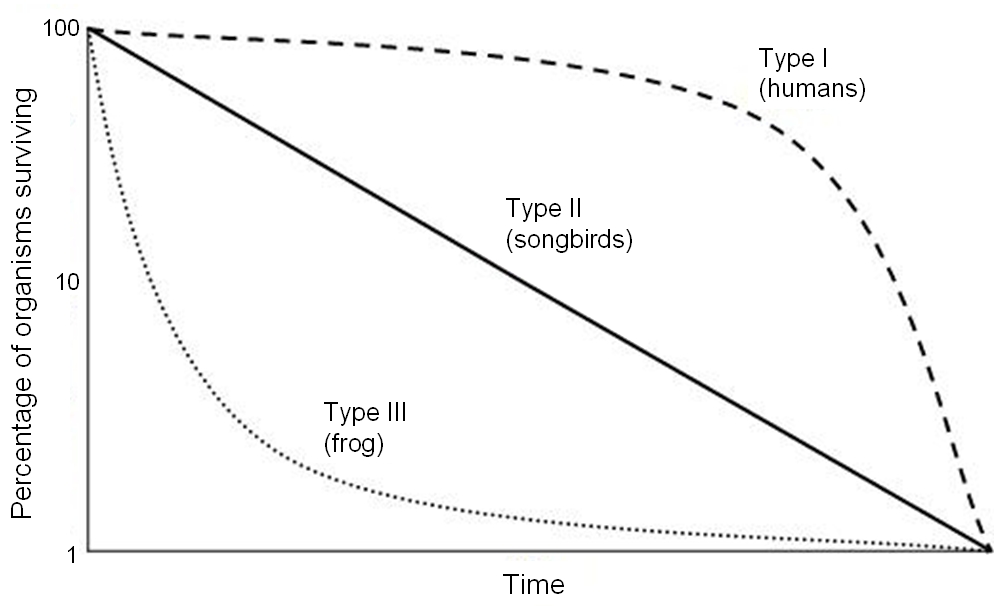
Type I Survivorship:
- Exhibits high survival rates during early and middle life.
- Mortality rates in a Type I survivorship curve increase steeply during old age.
- Link: Humans are an example of a K-selected species, and K-selected species generally exhibit a Type I survivorship curve. We invest heavily in our young, ensuring they survive to adulthood, but eventually, cellular senescence catches up with us.
Type II Survivorship:
- Exhibits a roughly constant mortality rate across all age classes. An individual is equally likely to die at any point in its life.
- Link: Songbirds frequently exhibit a Type II survivorship curve. A squirrel or a hawk is just as likely to eat a one-year-old songbird as a four-year-old songbird.
Type III Survivorship:
- Exhibits very high mortality rates for young individuals.
- Individuals surviving early life in a Type III survivorship curve experience high survival rates as adults.
- Link: r-selected species generally exhibit a Type III survivorship curve. Consider an oak tree or an oyster: 99.9% of acorns and larvae are eaten or destroyed immediately. But if an acorn manages to become a fully grown oak tree, it will likely survive for centuries.

When standing in front of a classroom, remind your students that the math of demography is simply nature's bookkeeping. Whether it is an r-selected dandelion exploiting a freshly disturbed patch of soil, or a logistic curve mapping a deer population hitting its environmental limit, biology is bounded by physics. By mastering these models, we learn how to read the ledger of life itself.