Basic Concepts of Probability
Not sure you’re ready?
Take the ~3-minute readiness diagnostic and see where you stand.
The universe is rarely entirely predictable, but its uncertainties are bound by rigid, beautiful laws. Probability is a mathematical measure of the likelihood that a specific event will occur. When we drop a glass, physics tells us it will shatter; but when we roll a die, the specific outcome is hidden behind a veil of chance. Yet, by understanding the mechanics of that chance, we can precisely quantify the unknown. This profound realization allows us to predict the aggregate behavior of chaotic systems, transforming pure guesswork into rigorous mathematical logic. For an educator mastering the Praxis Core, probability is not merely a collection of formulas; it is a framework for logical thinking that empowers you to teach students how to navigate an uncertain world.
To measure the unknown, we must first accurately map it. In any situation governed by chance, we begin by defining the boundary of possibilities. A sample space is the complete set of all possible distinct outcomes of an experiment. If you cannot describe the sample space, you cannot calculate probability. It is the absolute universe of whatever specific scenario you are analyzing.
Within that universe, we look for specific occurrences. An event is a defined set of outcomes resulting from a statistical experiment. When we specify what we are looking for, we are identifying our target. The outcomes that match our target have a special name: favorable outcomes are the specific outcomes from a sample space that satisfy the defined conditions of a target event.
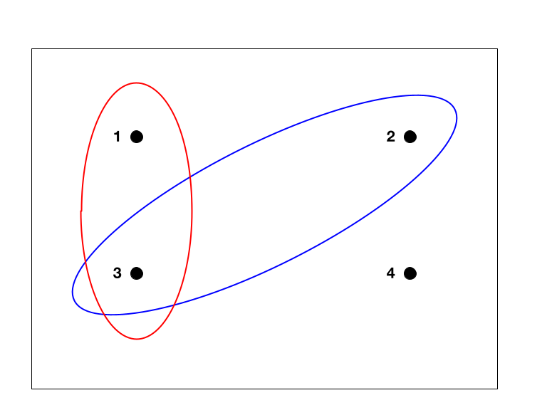
Sometimes, an event is complex, but the foundation of all probability rests on the simplest building blocks. A simple event is a mathematical event that consists of exactly one single outcome. For instance, rolling a specific number on a single die is a simple event, because it cannot be broken down into any smaller, more fundamental occurrences.
Once we have defined our universe (the sample space) and our target (the favorable outcomes), we can compute the likelihood of that target occurring.
The Fundamental Formula The theoretical probability of an event equals the number of favorable outcomes divided by the total number of possible outcomes.
Mathematically, this is expressed as: P(Event)=Total Number of Possible OutcomesNumber of Favorable Outcomes
However, this elegant formula harbors a hidden, critical requirement. Theoretical probability requires the assumption that all possible outcomes in a given sample space are equally likely to occur. If a die is weighted, or a coin is bent, the fundamental symmetry is broken, and our theoretical formula no longer accurately describes reality.

Probability is a tightly constrained measurement. Because it is fundamentally a ratio of a part to a whole, the probability of any event is mathematically restricted to a numerical value between 0 and 1, inclusive. It is impossible to have less than zero chance of something happening, and you cannot have more than a 100% guarantee.
- The Lower Bound: An event with a probability of exactly 0 is impossible and cannot occur. (e.g., Rolling a 7 on a standard six-sided die).
- The Upper Bound: An event with a probability of exactly 1 is absolutely certain to occur. (e.g., Rolling a number less than 10 on a standard six-sided die).
Because probabilities are ratios, they are highly flexible in how they can be written. A numerical probability value can be mathematically represented as a fraction, which perfectly preserves the exact ratio of favorable to total outcomes. Furthermore, a numerical probability value can be mathematically represented as a decimal, which makes it easy to compare different probabilities at a glance. Finally, a numerical probability value can be mathematically represented as a percentage, which is deeply intuitive for everyday understanding.
| Likelihood | Fraction Representation | Decimal Representation | Percentage Representation |
|---|---|---|---|
| Impossible | 0/6 | 0.00 | 0% |
| Even Chance | 1/2 | 0.50 | 50% |
| Certain | 52/52 | 1.00 | 100% |
To master basic probability, you must be intimately familiar with the mathematician’s favorite conceptual tools. These objects are perfectly symmetric, satisfying our requirement for "equally likely" outcomes. They are the classic laboratories of probability.
The Coin
The simplest generator of chance is the coin. A standard fair coin possesses exactly two distinct physical faces. In the universal language of probability, the two faces of a standard coin are universally referred to as heads and tails.
- Sample Space: {Heads, Tails}
- Total Outcomes: 2
The Die
Stepping up in complexity, we introduce the die. A standard fair six-sided die features the numerical values 1, 2, 3, 4, 5, and 6 on its respective faces.
- Sample Space: {1, 2, 3, 4, 5, 6}
- Total Outcomes: 6
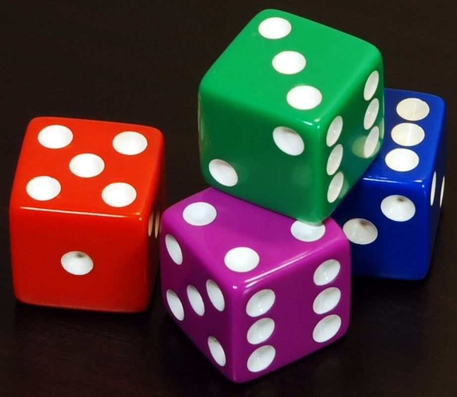
If we want to calculate the probability of the simple event "rolling a 4," there is exactly one favorable outcome out of six total possible outcomes. Thus, the theoretical probability is 1/6.
The Deck of Cards
The ultimate playground for discrete probability is the standard deck of cards. The arithmetic of playing cards is heavily tested on exams like the Praxis Core because of its structured internal symmetry.
- A standard deck of playing cards contains exactly 52 cards when jokers are excluded.
- A standard 52-card deck of playing cards is divided into exactly four equal suits.
- The four suits in a standard deck of playing cards are hearts, diamonds, clubs, and spades.
- Consequently, each individual suit in a standard 52-card deck of playing cards contains exactly 13 distinct cards (52÷4=13).
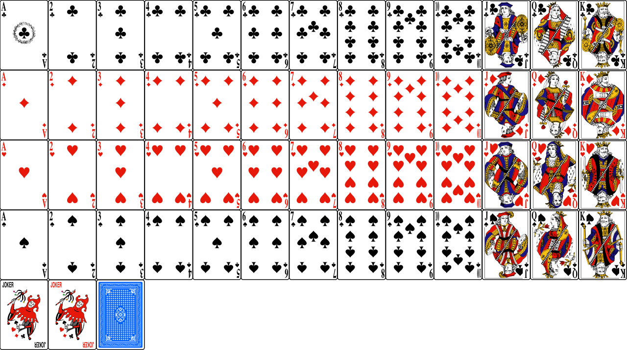
If you want to find the probability of drawing a "Heart", your favorable outcomes are 13, and your total possible outcomes are 52. The probability is 13/52, which simplifies to 1/4.
What happens when we account for every single possibility in our mathematical universe? Because the sample space represents everything that can possibly happen, the sum of the individual probabilities of all distinct possible outcomes within a single sample space equals exactly 1.
This leads us to a highly efficient mental shortcut: the complement.
The complement of an event includes every possible outcome in the sample space that does not belong to the target event. If our target event is "rolling a 1 or a 2," the complement is "rolling a 3, 4, 5, or 6."
Because the target event and its complement together make up the entire sample space, their probabilities must add up to 1. Therefore, the mathematical probability of the complement of an event equals 1 minus the probability of the target event occurring.
Complement Formula P(Complement)=1−P(Target Event)
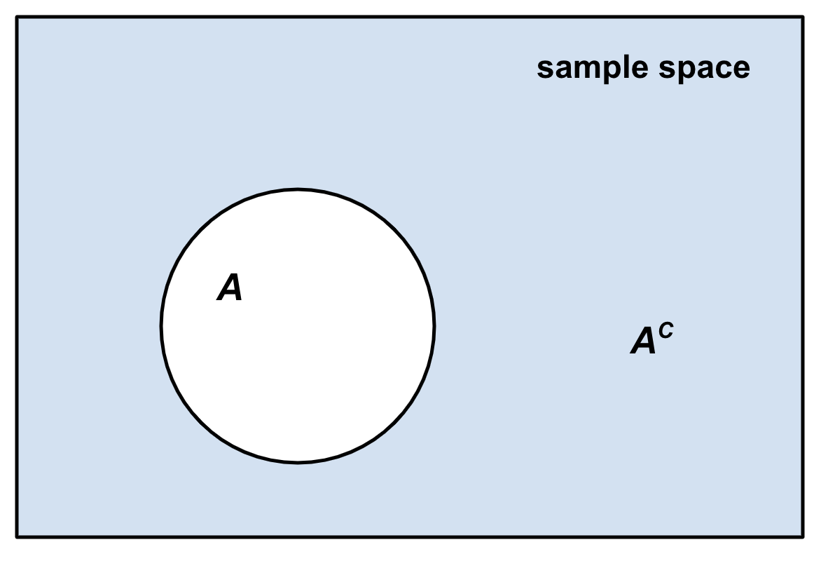
This is incredibly useful. If you know the probability of drawing a Heart is 1/4, you don't need to count the remaining cards to find the probability of not drawing a Heart. You simply calculate 1−(1/4)=3/4.
Thus far, we have lived in the world of pure, theoretical mathematics, assuming perfect symmetry. But probability can also be applied to messy, real-world data and continuous physical spaces.
Experimental Probability
When we lack a perfect theoretical model—or when we simply want to test reality—we turn to observation. Experimental probability is calculated by dividing the observed number of times an event occurred by the total number of trials conducted.
If you flip a coin 100 times, and it lands on heads 58 times, the experimental probability of heads in your trial is 58/100, or 58%. (Notice this differs from the theoretical probability of 50%). As you increase the number of trials, the experimental probability will reliably converge on the theoretical probability—a phenomenon known as the Law of Large Numbers.
Geometric Probability
Lastly, probability is not restricted to counting distinct, separate objects like cards or coins; it can also measure continuous physical space.
When dealing with a two-dimensional surface, like a dartboard or a shaded region of a circle, geometric probability calculates likelihood by dividing a specific target geometric area by the total available area. If a square target measuring 2 square feet sits inside a larger board measuring 10 square feet, the probability of a randomly thrown dart hitting the target is 2/10, or 20%.
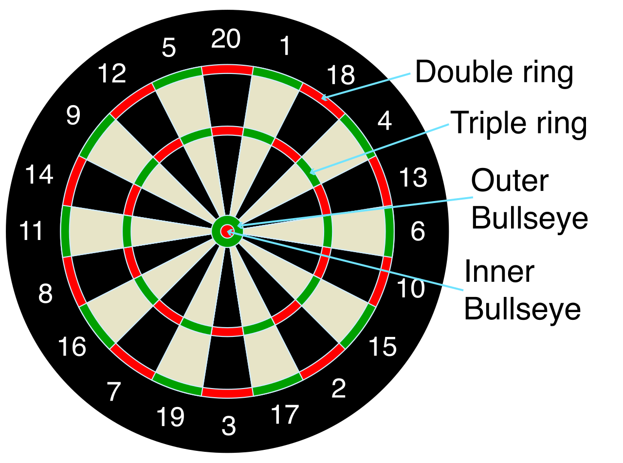
Similarly, in one dimension, geometric probability calculates likelihood by dividing a specific target geometric length by the total available length. If a 10-inch piece of string has a 3-inch section painted red, the probability that a random cut along the string happens in the red section is 3/10, or 30%.
Whether you are counting cards, tallying experimental coin tosses, or measuring the area of a target, the governing logic of probability remains gloriously the same: define your total universe of possibilities, isolate the specific conditions you care about, and measure the exact ratio between them.