Counting Techniques and Combinations
Not sure you’re ready?
Take the ~3-minute readiness diagnostic and see where you stand.
When we attempt to calculate the probability of a future occurrence, we must first map the entirety of what is possible. Counting, in the mathematical sense, is not merely tallying objects one by one; it is the systematic unearthing of hidden structures within sets of choices. It is the geometry of branching paths. Before we can determine how likely an event is, we must rigorously define the boundaries of the universe in which that event takes place.
To study outcomes, we first require a framework. In mathematics, the sample space of an experiment is the exhaustive set of all possible distinct outcomes. It is the absolute limit of what can happen in a given scenario. Within that universe, we look for specific occurrences. An event is a specific outcome or a defined set of outcomes within a larger sample space.
Consider the simplest engines of randomness. A standard coin flip generates exactly two possible outcomes: heads or tails. Our sample space has a size of two. If we look at a die, a standard number cube features exactly six distinct faces. Therefore, tossing a single standard number cube generates exactly six possible outcomes.
But what happens when the universe gets slightly more complicated? What if we toss a coin and roll a number cube?
Mapping the Branches: Tree Diagrams
To visualize compound choices, we use a geometric tool. A tree diagram represents all possible outcomes of a sequence of events by using branches to connect each initial choice to subsequent choices.
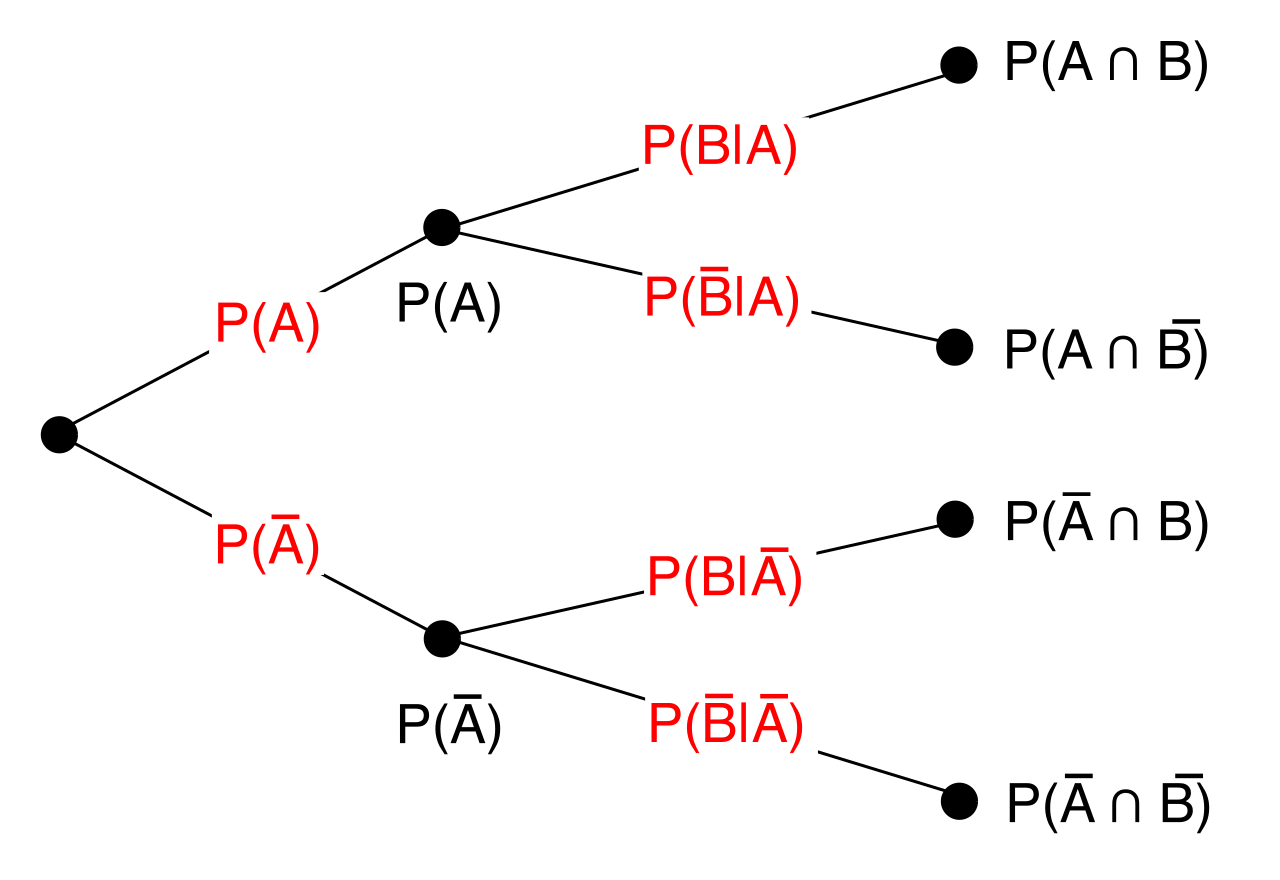
Imagine a starting point that splits into two branches: Heads and Tails. From the end of the Heads branch, six new branches sprout (1 through 6). From the Tails branch, another six sprout. By tracing every path from the root to the tip of the leaves, we see every distinct reality. By following this diagram, we find that tossing a standard coin and a standard number cube simultaneously generates exactly twelve possible outcomes (2×6=12).
Drawing a tree diagram is wonderfully intuitive, but it becomes agonizingly tedious as the number of events grows. Instead, we extract the mathematical essence of the tree diagram to create rules.
The Fundamental Counting Principle This principle dictates multiplying the number of choices for each successive independent event to find the total possible outcomes.
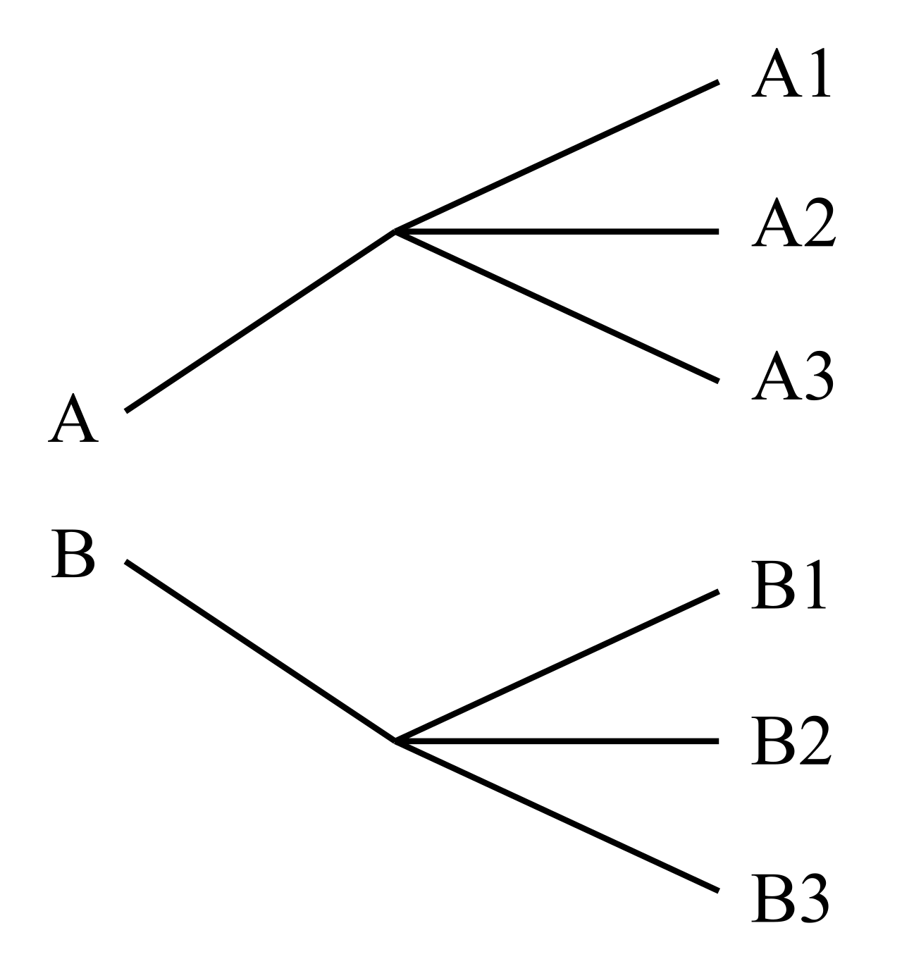
Because every branch of our first choice blossoms into a full set of secondary choices, multiplication is the natural shorthand.
- If you flip a coin twice, it is 2×2=4 outcomes.
- Flip it three times, 2×2×2=8.
- We can generalize this elegantly: The total number of outcomes for flipping a coin multiple times is calculated by raising two to the power of the number of flips (2n).
The exact same multiplication governs the rolling of number cubes:
- Tossing two standard number cubes simultaneously generates exactly thirty-six possible outcomes (6×6=36).
- Tossing three standard number cubes simultaneously generates exactly 216 possible outcomes (6×6×6=216).
The Addition Principle
There are moments, however, when choices are parallel rather than sequential. Suppose you are allowed to roll either one number cube or flip one coin, but not both. You are dealing with entirely separate timelines.
The Addition Principle This principle dictates adding the number of outcomes for mutually exclusive events to find the total possible outcomes.
What does it mean to be mutually exclusive? Mutually exclusive events are two or more specific events that cannot occur simultaneously. You cannot simultaneously pull a single card that is both an Ace and a King. If you are choosing one action from two mutually exclusive sets (6 die faces or 2 coin faces), your total sample space is 6+2=8 possible outcomes.
When navigating multiple events, we must ask a critical question: Does the first choice care about the second?
Independent events are events where the occurrence of one event does not affect the possible outcomes of the other events. A coin has no memory. If you flip ten heads in a row, the coin does not know this; the eleventh flip still has exactly two outcomes. The sample space remains rigid and unchanging.
However, many physical systems in reality do have memory. Dependent events are events where the occurrence of one event alters the total number of possible outcomes for subsequent events.
The Mechanics of Sampling
Nowhere is the distinction between independent and dependent events clearer than when drawing items from a finite pool—a process known as sampling.
| Condition | Mechanism | Mathematical Impact |
|---|---|---|
| Sampling with replacement | An item is returned to the selection pool before the next item is drawn. | Because the item goes back, it keeps the total number of available choices constant for each successive selection. These are independent events. |
| Sampling without replacement | A chosen item is removed from the selection pool permanently after being drawn. | Because the item is gone, it decreases the total number of available choices by exactly one for each successive selection. These are dependent events. |
Let us push sampling without replacement to its absolute limit. Suppose you have 5 different books and you want to arrange all of them on a shelf.
For the first slot on the shelf, you have 5 choices. For the second slot, you have 4 choices (one book is already placed). For the third, 3 choices. For the fourth, 2 choices. For the last, exactly 1 choice.
According to the Fundamental Counting Principle, we multiply these together: 5×4×3×2×1=120.
This descending multiplication occurs so frequently in probability that mathematicians gave it its own name and symbol.
Factorial A factorial represents the mathematical product of a positive integer and all the positive integers below that integer down to one.
The mathematical symbol for a factorial is an exclamation mark placed immediately after an integer (e.g., $5!$).
Before we move forward, we must address a brilliant, necessary quirk of mathematics. What happens if we have zero objects to arrange? The value of zero factorial is defined mathematically as exactly one ($0! = 1$). Why? Because there is exactly one way to arrange zero items: by doing nothing. The empty set has exactly one configuration.
We have arrived at the pinnacle of counting techniques. The Praxis exam will relentlessly test your ability to differentiate between two concepts: Permutations and Combinations. The entire difference rests on one word: Sequence.
Permutations (Order Matters)
A permutation is an arrangement of a specific number of items where the sequence of the items strictly matters.
Imagine assigning three unique titles—President, Vice President, and Treasurer—to three students chosen from a class of twenty. If Alice is President and Bob is Vice President, that is a profoundly different outcome than if Bob is President and Alice is Vice President. The sequence of the names creates a brand-new outcome.
Because of this, arranging distinct objects in a straight line utilizes permutation calculations because the specific sequence of objects changes the outcome.
The formula for finding the number of permutations of choosing k items from a pool of n items is: P(n,k)=(n−k)!n!
Combinations (Order is Irrelevant)
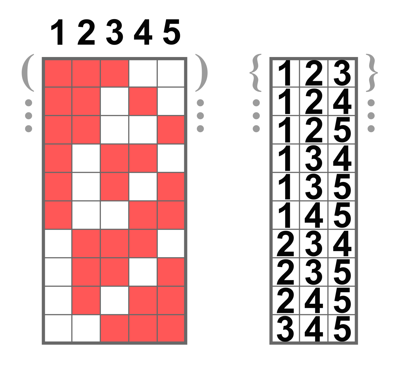
Now, imagine a different scenario. A combination is a selection of a specific number of items where the sequence of the items does not matter.
Suppose instead of electing officers, we are merely picking three students to serve on a cleanup crew. If I pick Alice, Bob, and Charlie, it is the exact same cleanup crew as picking Charlie, Bob, and Alice. The sequence does not create a new reality; it merely describes the same reality in a different way.
Because order does not generate unique outcomes here, forming a generalized committee from a larger group utilizes combination calculations because the specific order of selection is irrelevant.
Unifying the Two Concepts
If combinations ignore the different orderings of the same items, it stands to reason that combinations will always yield a smaller total number than permutations. In fact, the number of possible combinations for a subset of items is always less than or equal to the number of possible permutations for that same subset.
But how much smaller?
Think like a mathematician. Let's say we have already calculated the permutations for choosing 3 students from 20. We have counted every distinct arrangement. But wait—for any specific group of 3 students (say, Alice, Bob, and Charlie), how many different ways did we arrange them in our permutation count? We arranged them $3!$ ways (which is 6 ways). To convert our permutations into combinations, we must divide out this redundancy! We must group those 6 overlapping arrangements together and count them as just 1 combination.
The Combination Formula The formula for calculating combinations divides the total number of permutations by the factorial of the number of chosen items.
Mathematically, this elegant correction looks like this: C(n,k)=k!P(n,k)=k!(n−k)!n!
By dividing by k!, we effortlessly erase the illusion of order, leaving behind only the pure, unordered selections.
When you sit down to calculate outcomes on your exam, ask yourself these core questions: Are the events independent or dependent? Are we replacing the items or leaving them out? And, most importantly, does the order of the final result matter? Once you answer those, the geometry of possibility resolves itself into clear, calculable certainty.