Following Arithmetic and Algebraic Procedures
Not sure you’re ready?
Take the ~3-minute readiness diagnostic and see where you stand.
Mathematics, at its absolute core, is the study of inescapable rules. When we trace the path of a falling object, calculate the compounding interest in a bank account, or program a computer to sort data, we are observing systems relentlessly executing defined operations. To understand and predict these systems, we must learn to read their instruction manuals. This requires mastering the art of following arithmetic and algebraic procedures—not by rote memorization, but by understanding the precise sequence of steps, the conditional logic, and the recursive loops that dictate how numerical values evolve. A single misstep in precedence or a failure to track a variable's changing state will cascade into an entirely incorrect conclusion.
In the Praxis Core Mathematics exam, your ability to follow procedures is tested through algebraic manipulation, algorithmic flowcharts, and recursive sequences. Let us dissect how to navigate these logical structures with absolute precision.
Fundamentally, an algebraic procedure is a sequence of defined mathematical operations applied to an initial value. You can think of it as a factory assembly line. Raw materials (numbers) enter the line, and a strict sequence of machines (operations) transforms them into a final product.
When you encounter an expression like 3(x+2)2−5, it is completely inert until you provide an input. Substitution involves replacing variables in an algebraic expression with specific numerical values. Once the abstract letters become concrete numbers, the machinery turns on. At this stage, evaluating an expression requires applying arithmetic operations after substituting variables with numbers.
However, the sequence in which these operations fire is not arbitrary. If two people evaluate the same expression but perform the operations in different orders, they will get different results. To prevent mathematical chaos, we rely on a universal agreement.
The Universal Grammar: Order of Operations
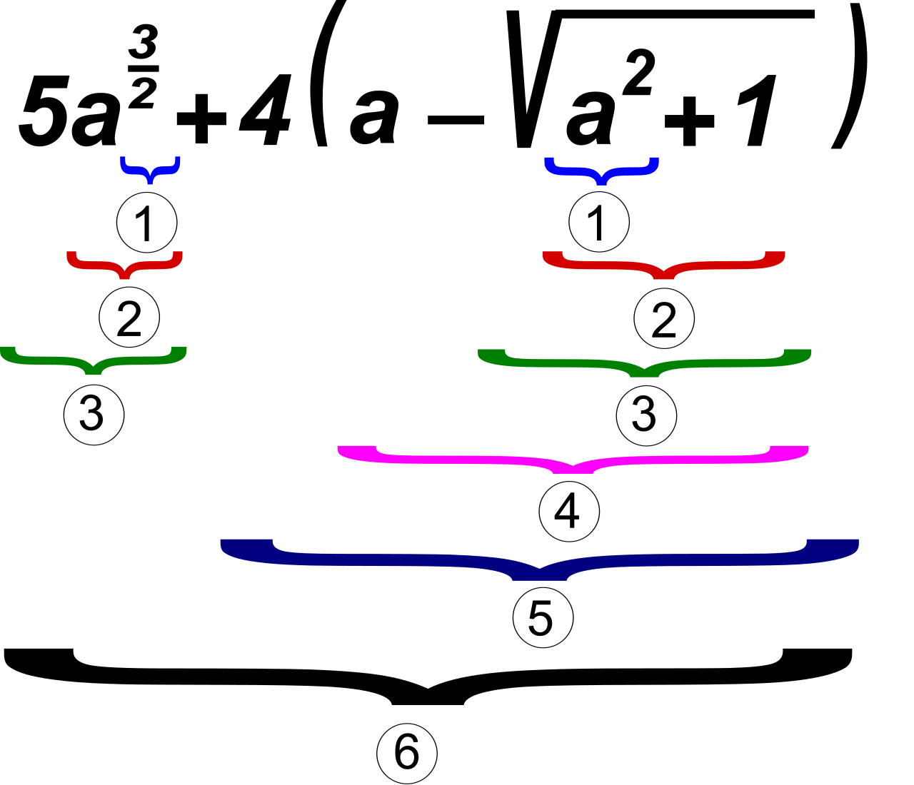
The order of operations is the strict hierarchy that governs how mathematical sentences are read and executed.
The Hierarchy of Execution
- The order of operations dictates that expressions inside parentheses are evaluated first. Parentheses act as an override switch, forcing you to resolve whatever is enclosed before looking at the rest of the expression.
- The order of operations dictates that exponents are evaluated before multiplication and division. Exponents (and roots) represent rapid, repeated multiplication, so they carry a higher priority than single instances of multiplication.
- The order of operations dictates that multiplication and division are evaluated before addition and subtraction.
Working left to right within these hierarchical tiers ensures that every algebraic procedure yields one unambiguous answer.
Running the Machine in Reverse: Solving Equations
Evaluating an expression is running the mathematical machinery forward. Solving an equation is running it in reverse. If you know the final output of a procedure and need to discover the initial input, you must systematically undo every step.
This is achieved using inverse operations. An inverse operation reverses the effect of another specific mathematical operation. Addition undoes subtraction; division undoes multiplication; a square root undoes a square.
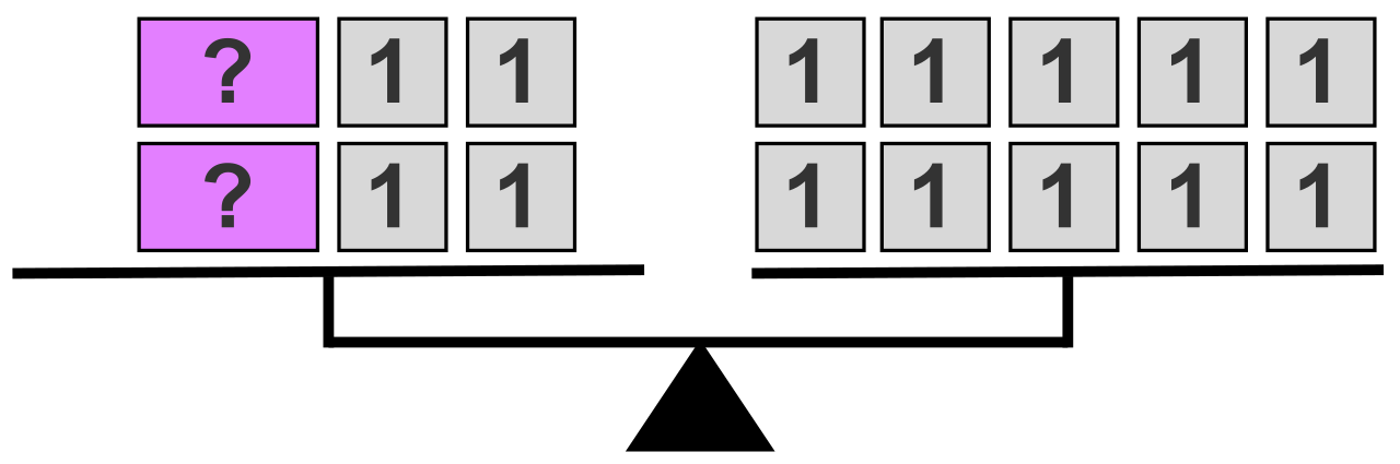
Solving an equation step-by-step requires applying inverse operations to both sides of the equation. Why both sides? An equation is a statement of perfect balance. Maintaining equality requires performing the exact same mathematical operation on both sides of an equation. If you divide the left side of a scale by two without dividing the right side by two, the equality shatters.
In many fields—particularly computer science and systems engineering—algebraic procedures are not written as horizontal equations, but as visual diagrams. A flowchart is a visual representation of a step-by-step mathematical algorithm. It maps the precise flow of logic from the start of a process to its conclusion.
To read a flowchart, you must understand its standard morphology. The shapes themselves communicate the nature of the instruction.
| Shape | Meaning in a Flowchart |
|---|---|
| Oval | In standard algorithmic flowcharts, oval shapes indicate the start point or end point of a process. They act as the terminal boundaries of the algorithm. |
| Rectangle | In standard algorithmic flowcharts, rectangular shapes represent processing steps or mathematical operations. This is where the actual arithmetic (e.g., "Add 5 to X") occurs. |
| Diamond | In standard algorithmic flowcharts, diamond shapes denote decision points or conditional branching. These ask a question, usually resulting in a "Yes/No" or "True/False" answer. |
Branching and Looping
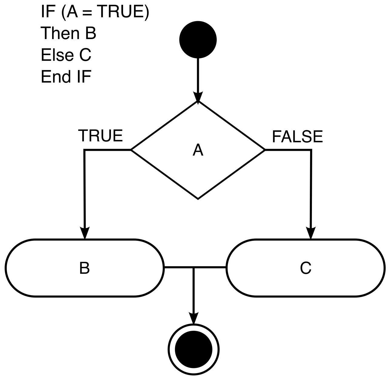
The diamond shape introduces dynamic behavior into an otherwise static list of instructions. A conditional branch in a flowchart directs a process along different paths based on a true or false condition. Imagine a train arriving at a switch on the tracks: if the train is carrying freight (True), it goes left to the warehouse; if it is carrying passengers (False), it goes right to the station.
Often, conditional branches force a process to repeat. A loop in a flowchart repeats a specific sequence of operations until a defined condition is met. For example, an algorithm might subtract 10 from a starting value and loop back to do it again until the value drops below zero.
How to Trace an Algorithm
On the Praxis exam, you will be asked to determine the final output of a given flowchart. Do not attempt to hold changing values in your head. The human brain is a terrible scratchpad for transient data.
Tracing an algorithm requires recording the current value of all variables after every individual operation. The professional method is to draw a "Trace Table."
Imagine an algorithm with two variables, A and B. Every time you pass through a rectangle in the flowchart, cross out the old value in your table and write the new one. If the algorithm loops three times, you should have three distinct updates recorded. This mechanical bookkeeping is the only way to guarantee accuracy when following complex algorithmic procedures.
Algorithms often produce sequences of numbers. While some sequences can be calculated directly (using an explicit formula), others force you to build each step upon the foundation of the last.
A recurrence relation is a mathematical equation that expresses the nth term of a sequence as a function of previous terms. When a sequence is governed by such an equation, we call it recursive. A recursive sequence defines each term based on one or more previous terms in the sequence.
To understand recursion, picture a staircase. To stand on the 10th step, you must first reach the 9th step. To reach the 9th, you must reach the 8th. Because every term relies on the preceding one, a recursive sequence requires at least one initial starting value known as the base case. Without a base case (the ground floor), the sequence can never begin.
Common Types of Sequences
Mathematical procedures often generate distinct patterns depending on the operations used to step from one term to the next.
- Arithmetic Sequences: An arithmetic sequence adds a constant numerical difference to the previous term to generate the next term. If your base case is 3 and your constant difference is +4, your sequence is 3,7,11,15,… It grows in a perfectly straight line.
- Geometric Sequences: A geometric sequence multiplies the previous term by a constant numerical ratio to generate the next term. If your base case is 3 and your constant ratio is ×2, your sequence is 3,6,12,24,… It experiences compounding, exponential growth.
The Ultimate Recursive Pattern: The Fibonacci Sequence
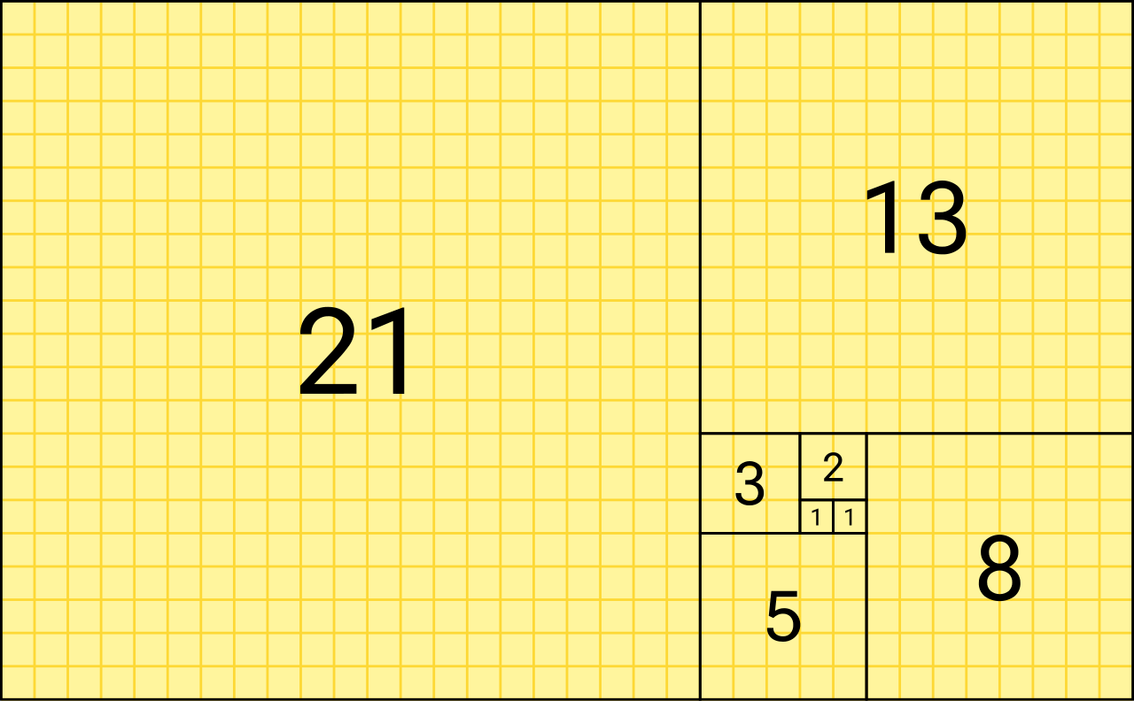
Nature itself is deeply recursive. The branching of trees, the spirals of shells, and the breeding patterns of animals often follow a very specific recursive logic. The Fibonacci sequence is a mathematical recursive sequence that frequently appears in the natural world.
Unlike a simple arithmetic or geometric progression that looks back at only one previous term, the Fibonacci sequence adds the two immediately preceding terms to generate the next term.
Because it requires two preceding terms, it needs two base cases: 0 and 1.
- 0+1=1
- 1+1=2
- 1+2=3
- 2+3=5
The sequence emerges as: 0,1,1,2,3,5,8,13,21,…
The Drawback of Recursion
Recursive procedures are elegant, but they hide a computational burden. Finding a specific term in a recursive sequence requires calculating all intermediate preceding terms.
If you are asked to find the 50th term of an arithmetic sequence explicitly, you can just plug 50 into a formula. But if you are asked to find the 50th Fibonacci number, you cannot skip ahead; you must patiently calculate the 3rd, 4th, 5th, and so on, all the way to the 49th term.
This brings us full circle. Whether you are substituting values into an algebraic expression, tracing variables through a looping flowchart, or building a sequence step-by-step from a base case, the fundamental skill remains exactly the same. You must respect the order of operations, maintain rigorous written records of changing values, and trust the procedural logic above your own intuition. That is how you master mathematical mechanics.