Reading and Interpreting Bar and Line Graphs
Not sure you’re ready?
Take the ~3-minute readiness diagnostic and see where you stand.
Staring at a raw table of data is much like staring at a sheet of complex musical notation. You might recognize the individual numbers just as you recognize individual notes on a staff, but grasping the overarching melody—the sudden spikes, the steady declines, the comparative magnitudes—requires a strenuous mental translation. Visual displays of quantitative data act as the instruments that play the music of mathematics. They take dense, abstract tables and map them onto physical, spatial dimensions, transforming a tedious chore of arithmetic into an immediate, intuitive realization of truth.
When you sit down to tackle the data interpretation questions on the Praxis Core Mathematics exam, you are essentially acting as a translator. Your job is to look at spatial relationships—the length of a rectangle, the tilt of a line segment—and accurately translate them back into numerical facts.
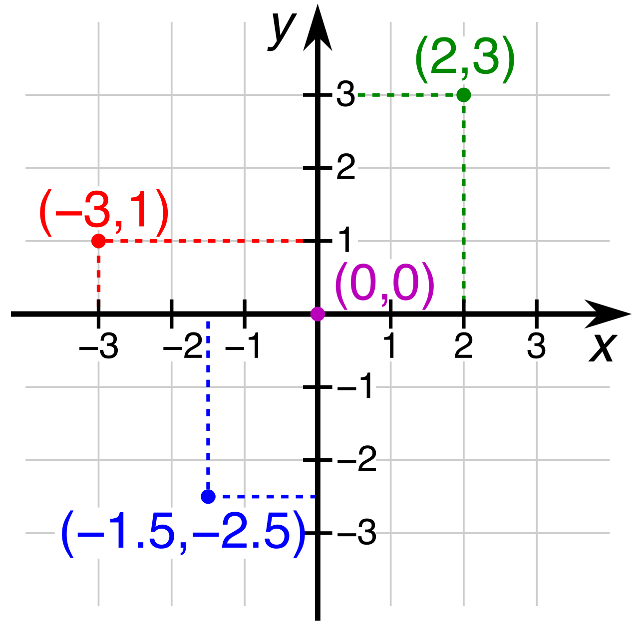
Before we can read the music, we must understand the stage upon which it is performed. Every well-constructed mathematical graph possesses a foundational anatomy designed to orient the reader.
The first thing you must read is the title. The title of a mathematical graph explicitly describes the overall subject matter being depicted. But more fundamentally, the title of a mathematical graph explicitly describes the relationship between the plotted variables. It tells you exactly what conversation the two axes are having with one another.
The framework itself is anchored by the origin, which is the specific coordinate point where the horizontal axis and the vertical axis intersect on a graph. From this zero point, the axes branch outward. Whenever a graph maps several different variables simultaneously, you will see a legend. A legend provides the definitions for different colors, patterns, or line styles utilized within a graph, ensuring you know exactly which entity each visual element represents.
The Danger of the Scale Break
Sometimes, all the fascinating data happens far away from zero. For example, if we are graphing human body temperature, everything of interest occurs between 95°F and 105°F. Plotting a graph starting precisely from zero would compress all the relevant data into a microscopic, unreadable sliver at the very top of the page.
To solve this, mathematicians use a scale break. A scale break indicates that a continuous portion of the numerical axis has been visually omitted to save space. Scale breaks are frequently represented by a jagged zigzag line drawn directly on the affected axis.
Warning: Failing to account for a scale break on an axis can cause a reader to visually misjudge the actual mathematical proportions between plotted values.
If Bar A is twice as tall as Bar B visually, but the axis has a scale break that jumps from 0 to 100, Bar A might actually represent 120 and Bar B might represent 110. The visual "double height" is an optical illusion created by the omitted space. Always read the axis numbers!
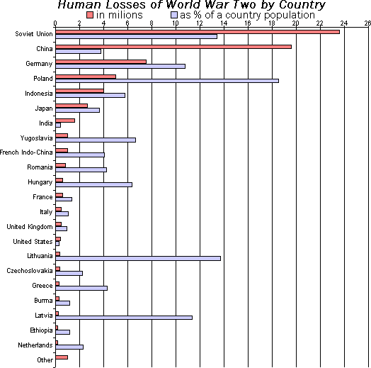
When the goal is to compare distinct, non-overlapping bins of data, we rely on the bar graph. A bar graph uses rectangular bars to represent the frequencies or values of discrete categories. "Discrete" simply means separate and distinct—such as months of the year, types of automobiles, or different school districts.
The cardinal rule of reading this chart is that geometry is a strict proxy for quantity: the length of each bar in a bar graph is directly proportional to the numerical value that specific bar represents.
Bar graphs can be oriented with bars running either vertically or horizontally. On the Praxis exam, you will most commonly encounter the vertical orientation. In this layout, the horizontal axis of a vertical bar graph typically denotes the distinct categories being compared, while the vertical axis of a vertical bar graph typically denotes the continuous numerical scale for the quantities being measured.
Extracting Data from Bars
Because length dictates value, comparing the heights of different bars in a bar graph visually reveals which categories have the largest and smallest absolute values in a fraction of a second. The tallest bar is the maximum; the shortest bar is the minimum.
When you need to find the exact mathematical difference between two categories, you must rely on the vertical axis. To find the quantitative difference between two categories on a bar graph, a reader subtracts the numerical value of the smaller bar from the numerical value of the larger bar.
Complex Comparisons: Grouped and Stacked Bars
Sometimes, a single category contains multitudes. If we are comparing the revenue of three different bakeries, we might also want to know how much of that revenue comes from cakes versus pastries.
- Grouped Bar Graphs: A grouped bar graph displays multiple bars side-by-side for each distinct category to facilitate sub-group comparisons. You might see two bars over "Bakery A"—one blue for cakes, one red for pastries.
- Stacked Bar Graphs: A stacked bar graph divides a single vertical or horizontal bar into separate segments. Rather than sitting side-by-side, the cake and pastry revenues are stacked vertically into a single column. The total height of the bar represents the bakery's total revenue, and each segment within a stacked bar graph shows the relative contribution of a sub-group to the total category value.
While bar graphs excel at comparing isolated categories, they are terrible at showing a continuous flow. For that, we use the line graph.
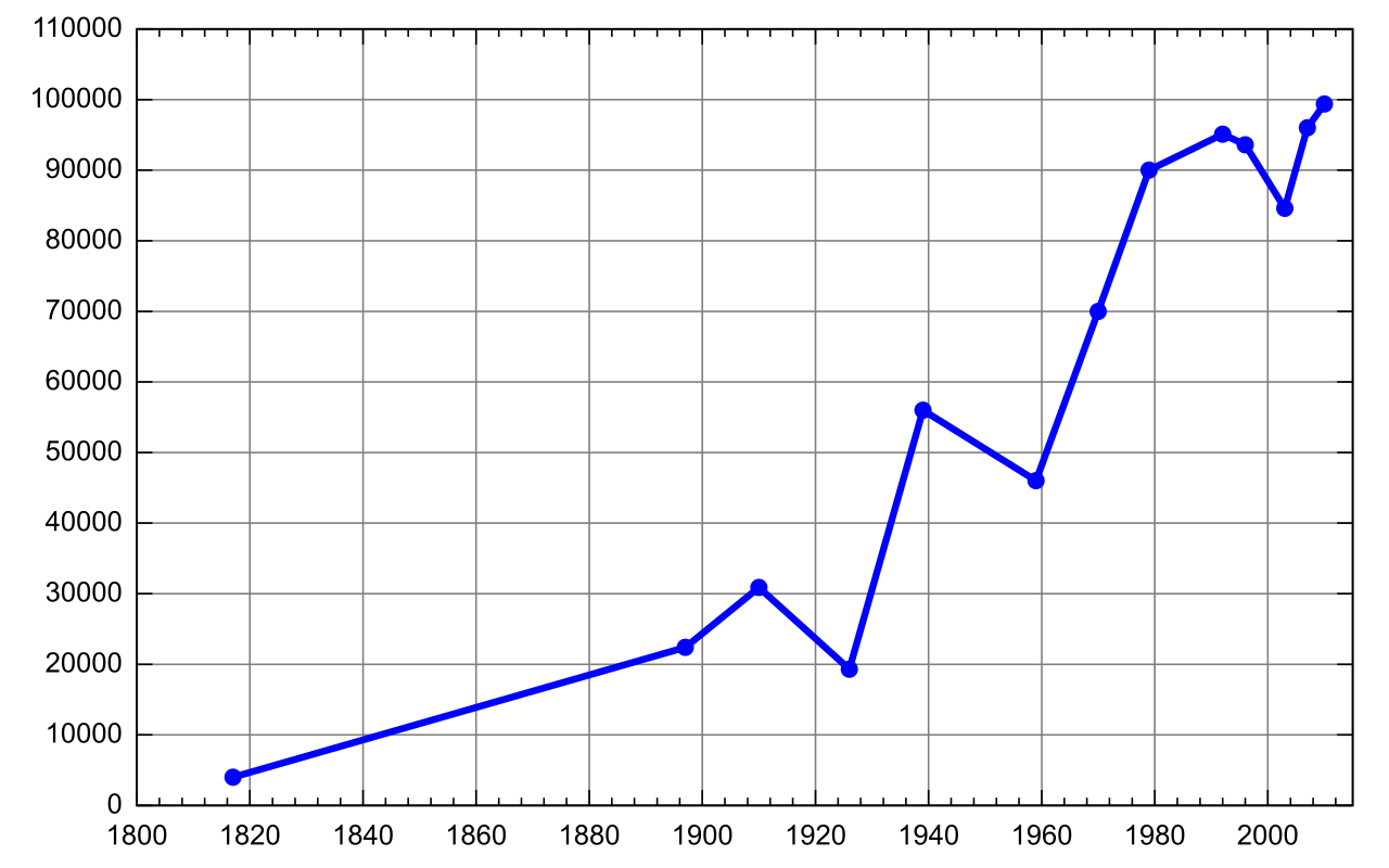
A line graph uses individual data points connected by straight line segments to represent quantitative data. Above all else, line graphs are primarily used to display how a specific numerical variable changes over a continuous progression of time.
The axes here are highly standardized. The horizontal axis of a line graph almost always represents chronological time intervals (such as hours, days, or years). Meanwhile, the vertical axis of a line graph represents the numerical value of the specific quantitative variable being tracked over time (such as temperature, population, or bank account balance).
Decoding Slopes and Rates of Change
The true power of a line graph lies not in the dots themselves, but in the segments connecting them. The tilt of these lines immediately translates into behavioral trends:
- Upward Trends: An upward-sloping line segment on a line graph indicates an increase in the measured numerical value during that specific time interval.
- Downward Trends: A downward-sloping line segment on a line graph indicates a decrease in the measured numerical value during that specific time interval.
- Stagnation: A perfectly horizontal line segment on a line graph indicates that the measured numerical value remained constant during that specific time interval.
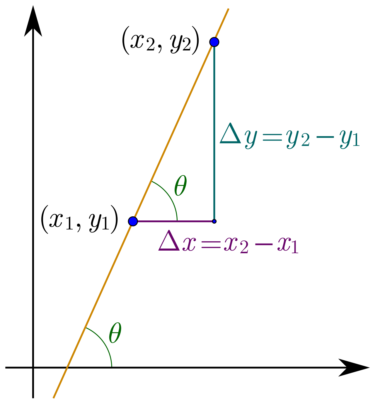
Even more importantly, the line graph reveals velocity. The steepness of a line segment on a line graph visually represents the rate of change of the measured variable.
- A steeper slope on a line graph indicates a faster rate of mathematical change. (A sharp spike upwards means a sudden explosion in value).
- A flatter slope on a line graph indicates a slower rate of mathematical change. (A gentle drift upwards means gradual growth).
Just as we can group bar graphs, multiple distinct lines can be plotted on the same line graph to compare data trends among different entities over the identical time period. For example, graphing the stock prices of two competing companies over a decade allows you to instantly see when one surged past the other.
Because line graphs plot variables that exist on a continuous spectrum, they grant us a special mathematical superpower: the ability to estimate data that we did not actually measure.
Interpolation
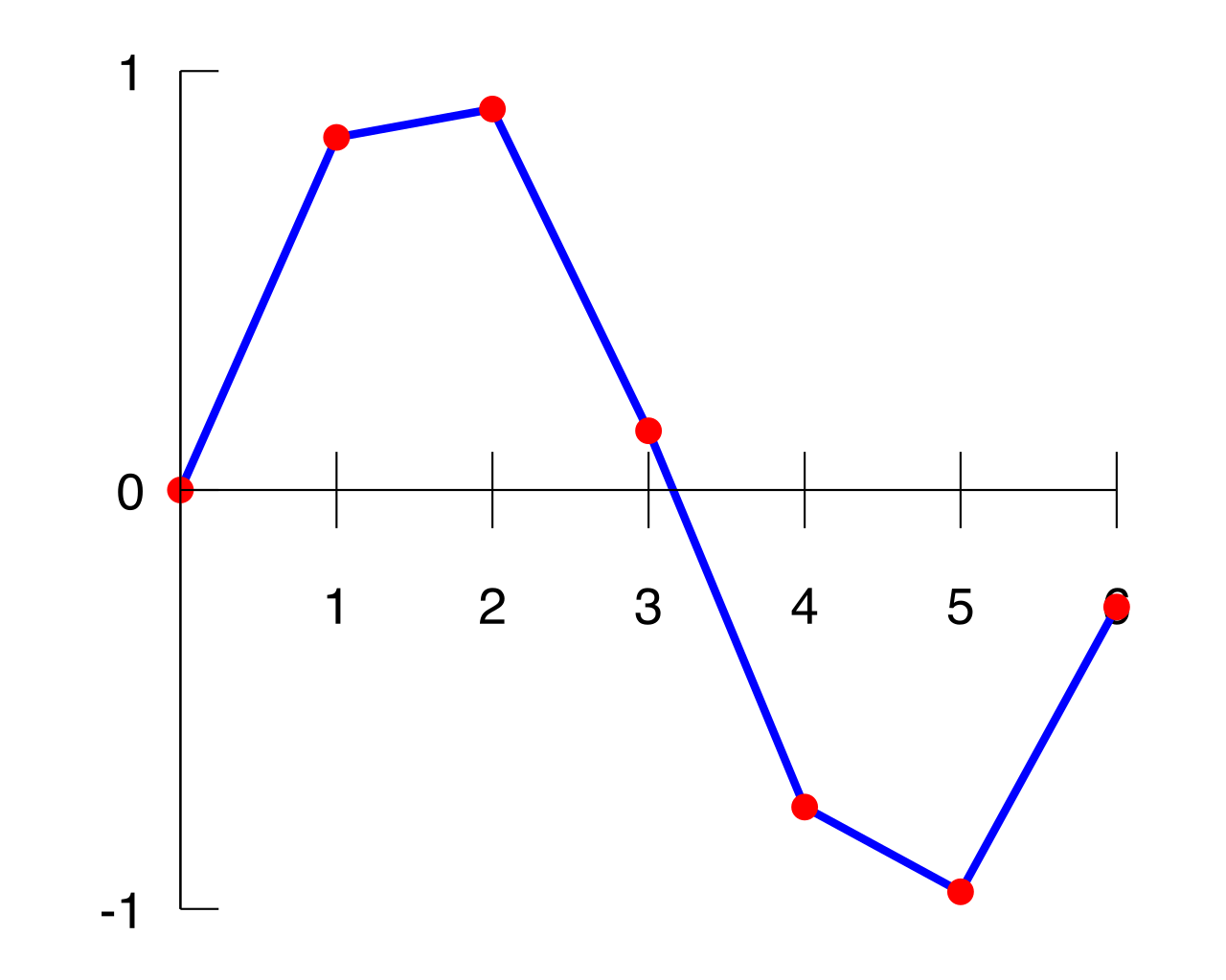
If a scientist records a chemical's temperature at 1:00 PM and again at 3:00 PM, they have two dots. By connecting them with a straight line, they can look at where the line passes through the 2:00 PM mark. Interpolation on a line graph involves estimating a missing numerical value mathematically positioned between two explicitly plotted data points. You are looking inside the established bounds of your data.
Extrapolation
What if that same scientist wants to predict the temperature at 4:00 PM? They can extend the line's current trajectory outward into the future. Extrapolation on a line graph involves predicting a future numerical value mathematically positioned outside the range of existing plotted data points.
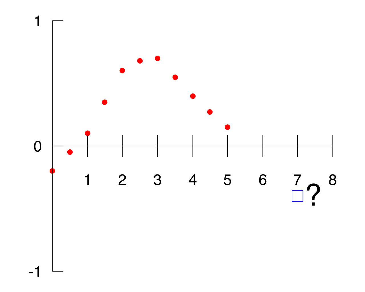
A word of caution on Extrapolation: While interpolation is usually quite safe, extrapolation assumes that the current mathematical trend will continue indefinitely. If a startup company's revenue goes from 1,000to2,000 to 4,000overthreemonths,extrapolationmightpredict8,000 for month four. But reality rarely follows a perfectly straight line forever.
To solidify your understanding for the Praxis exam, keep this fundamental distinction in mind:
| Feature | Bar Graphs | Line Graphs |
|---|---|---|
| Primary Purpose | Comparing absolute sizes of distinct categories. | Showing trends and continuous changes over time. |
| Horizontal Axis | Typically discrete, independent categories (e.g., Red, Blue, Green). | Almost strictly chronological time (e.g., 2020, 2021, 2022). |
| Visual Indicator of Value | The physical length or height of the rectangular bar. | The vertical position of the point on the grid. |
| Visual Indicator of Change | The quantitative difference calculated by subtracting bar heights. | The slope and steepness of the connecting segments. |
Mastering the translation between visual geometry and numerical reality will not only secure your success on the Praxis Mathematics exam, but it will fundamentally change the way you consume data in the world around you. You will no longer just read the numbers; you will hear the music.