Reading and Interpreting Data Tables and Charts
Not sure you’re ready?
Take the ~3-minute readiness diagnostic and see where you stand.
Nature presents herself to us in a state of sheer, overwhelming chaos. A biologist counting genetic traits in thousands of fruit flies, an educator tracking student test scores across a decade, or an economist analyzing shifting global markets—all are confronted with a deluge of raw information. To understand the universe, or even just a single classroom, we cannot simply stare at a chaotic pile of numbers. We must impose order. We must build a structure that allows patterns to emerge visibly and unmistakably. This is the fundamental purpose of organizing data into tables and charts. They are not mere bookkeeping devices; they are the lenses through which we focus the blur of reality into sharp, actionable mathematical truth.
To begin extracting meaning from raw data, we first have to understand the physical geometry of how we store it. At its core, a data table is a systematic arrangement of quantitative or qualitative information organized into rows and columns. It is a coordinate system for facts.
Think of a data table as a rigid grid.
- A row is a horizontal line of data entries within a table.
- A column is a vertical line of data entries within a table.
Where these two orthogonal lines cross, we find the fundamental unit of information: the cell. A cell is the precise intersection of a single row and a single column in a table. It is the box that holds the exact piece of reality we are trying to measure. A cell in a data table contains a specific data value corresponding to the intersection of its row and column headers.
But numbers floating in cells are meaningless without context. The number "42" could represent degrees Celsius, the number of passing students, or thousands of dollars. We give data context through table headers. These are descriptive labels located at the top of columns or the beginning of rows. Table headers identify the specific categories or units of measurement for the data within the corresponding rows or columns.
Extracting Data: Extracting a specific data point from a table requires locating the exact intersection of the relevant row header and column header. You sweep your eyes across the row and down the column until they meet. The cell at that intersection holds your answer.
Operating on the Grid: Differences and Ratios
Tables are not meant to be passively viewed; they are meant to be actively analyzed. Once we can extract data, we can manipulate it to uncover relationships.
Data tables are frequently utilized to determine differences between categories. If you want to know how much student enrollment grew between two years, you determine this by subtracting the numerical value in one cell from the numerical value in another cell.
Similarly, data tables are utilized to establish mathematical ratios. If you want to know the proportion of a school's budget spent on textbooks compared to technology, you determine this by dividing the numerical value in one cell by the numerical value in another cell. You are bringing two distant points on the grid into mathematical relationship with each other.
Often, data isn't a collection of unique, continuous numbers, but rather a chaotic pile of repeating categories. Imagine standing in a hallway and asking every passing student their favorite subject. You will hear "Math," "Science," "History," and "English" repeated over and over. To make sense of this, we build a frequency chart.
A frequency chart is a tabular data display showing how often each unique value or category occurs in a specific dataset.
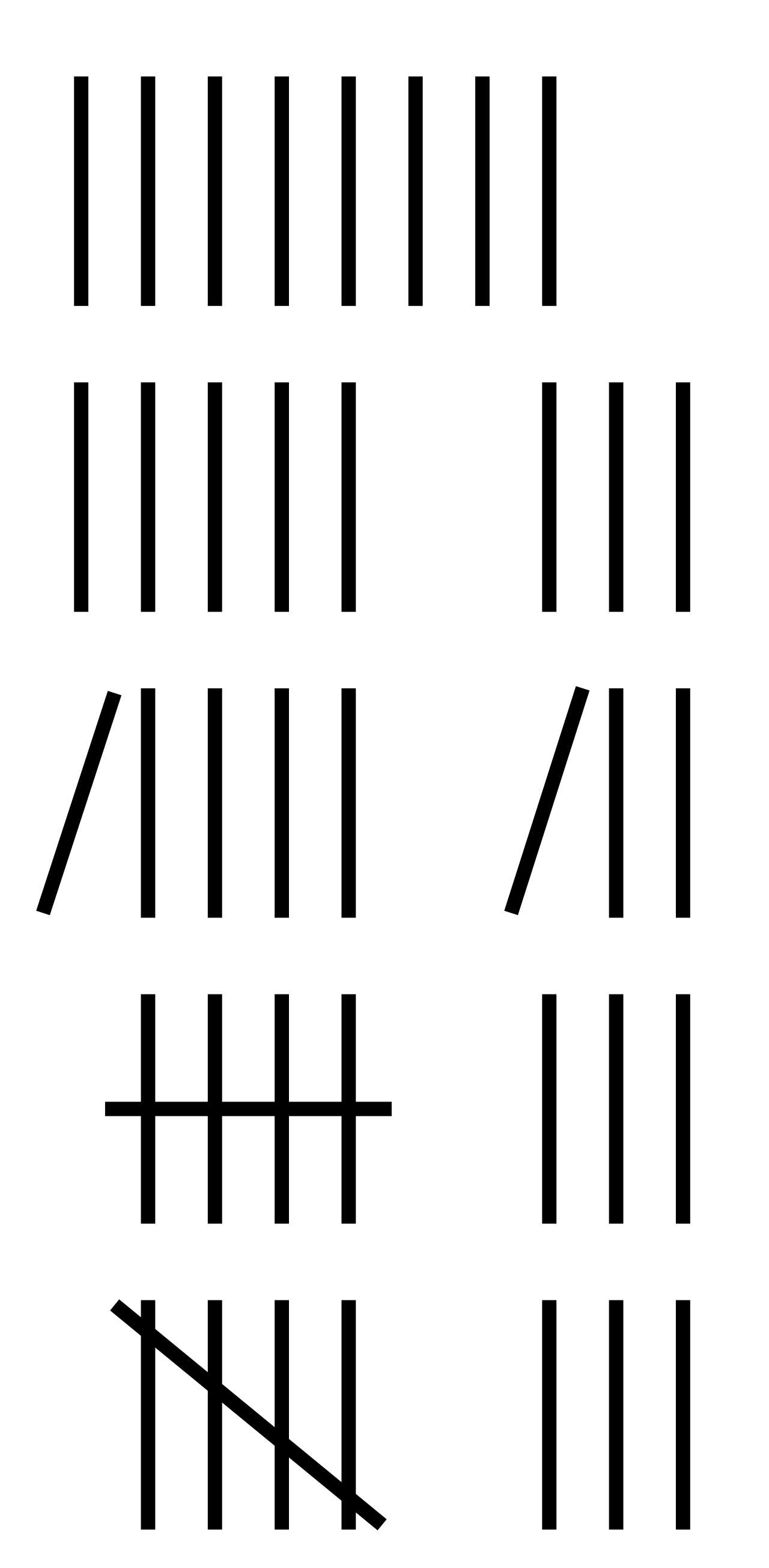
Frequency refers to the exact number of times a specific data value or category appears in a given dataset. When collecting this data in real-time by hand, educators and scientists often use tally marks, which are individual vertical strokes used in frequency charts to record and count occurrences of data points. Because human eyes struggle to quickly count large blocks of identical vertical lines, a standard grouping of tally marks consists of four vertical lines crossed by one diagonal line to represent the number five.
Once the data collection is complete, the total number of observations in a frequency chart is calculated by summing all the individual frequencies listed in the chart.
Contextualizing Counts: Relative and Cumulative Frequency
Knowing that 20 students prefer Math is an absolute fact, but it lacks context. Are there 25 students in the school, or 2,500? To solve this, we scale our frequencies.
Relative frequency is the mathematical ratio of a specific category's frequency to the total number of observations in the dataset. Because it is a ratio, relative frequency can be mathematically expressed as a fraction, a decimal, or a percentage. If 20 out of 100 students prefer math, the relative frequency is 10020, 0.20, or 20%. This allows us to compare datasets of entirely different sizes on equal footing.
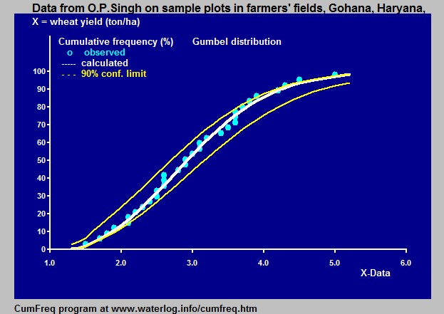
Sometimes, we care not just about isolated categories, but about the accumulation of data. Cumulative frequency is the running total of frequencies from the lowest recorded category up to a specific designated category. If you organize test scores from lowest to highest, the cumulative frequency at the "C" grade category tells you exactly how many students scored a "C" or worse. It provides an immediate snapshot of the data's progression.
Life is rarely so simple that a single variable tells the whole story. What if we want to observe two things at once to see if they are linked? For example, does participating in an after-school tutoring program affect whether a student passes a standardized test?
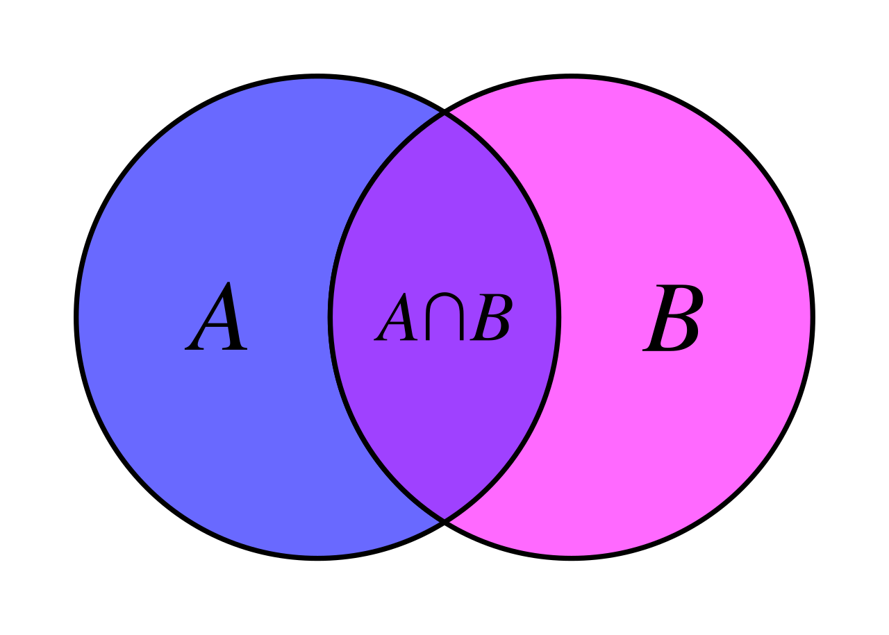
To investigate this, we use a two-way frequency table. This is a powerful matrix that displays the corresponding frequencies for two different categorical variables collected from the exact same subjects.
Let us look at the beautiful, rigid anatomy of a two-way frequency table:
| Passed Exam | Failed Exam | Total | |
|---|---|---|---|
| Attended Tutoring | 45 | 5 | 50 |
| Did Not Attend | 30 | 20 | 50 |
| Total | 75 | 25 | 100 |
There are three distinct regions in this table, each carrying specific mathematical weight:
- Joint Frequencies: These are the individual numerical counts located in the interior cells of a two-way frequency table. They represent the "joints" where the two variables intersect. In our table, the number 45 is a joint frequency—it counts the exact number of students who both attended tutoring and passed the exam.
- Marginal Frequencies: These are the overall row totals and column totals located in the outer margins of a two-way frequency table. They isolate a single variable, ignoring the other. The marginal frequency of 75 tells us how many total students passed the exam, entirely regardless of their tutoring status.
- The Grand Total: Located in the bottom right corner, the grand total represents the absolute scope of the dataset. There is a built-in mathematical symmetry here: the grand total in a two-way frequency table is calculated by summing all of the marginal row frequencies (50+50=100). Equivalently, the grand total in a two-way frequency table is also calculated by summing all of the marginal column frequencies (75+25=100).
Deducing the Unseen: The rigid arithmetic rules of a two-way table make it an elegant puzzle. Because the internal cells must sum to the margins, and the margins must sum to the grand total, a missing value in a frequency table with a known grand total is determined by subtracting the sum of the known frequencies from the grand total (or the respective marginal total).
If a coffee stain obscured the number of students who failed the exam without attending tutoring, you could simply take the marginal row total (50) and subtract the known joint frequency of students who passed without tutoring (30) to arrive back at 20. The structure of the table protects the integrity of the data.
When you sit down to interpret a data table or a frequency chart on an exam, do not view it merely as a block of text. View it as a mechanical system. Locate the headers to understand the units, navigate the intersections to extract the facts, and apply the arithmetic of differences, ratios, and relative frequencies to uncover the relationships hiding within the grid.