The Coordinate Plane and Linear Graphs
Not sure you’re ready?
Take the ~3-minute readiness diagnostic and see where you stand.
Legend has it that in the 17th century, the mathematician René Descartes, confined to his bed by illness, watched a fly crawling across the ceiling. He realized that he could describe the fly's exact, dynamic position at any given moment using nothing but its distances from two intersecting walls. Whether this specific anecdote is perfectly historical or a mathematically romantic myth, the machinery it birthed—the Cartesian coordinate system—is arguably the single greatest conceptual bridge in mathematical history. Before this innovation, algebra and geometry were completely isolated domains. Algebra was the manipulation of abstract symbols; geometry was the study of tangible shapes. By overlaying a grid of numbers onto physical space, the coordinate plane translates the continuous, visual world of geometry perfectly into the discrete, symbolic world of algebra. Every straight line becomes an equation; every algebraic relationship becomes a visible trajectory. To master the coordinate plane is to master the universal language of spatial and mathematical reality.

To describe space mathematically, we must first establish a reference frame. The Cartesian coordinate system consists of a horizontal number line and a vertical number line that intersect perfectly at a right angle.
The horizontal number line in a Cartesian coordinate system is called the x-axis. The vertical number line is called the y-axis.
The fundamental anchor of this entire system—the point where the x-axis and the y-axis intersect—is called the origin. Because this point represents zero movement in any direction, the coordinates of the origin on a Cartesian coordinate plane are always exactly (0,0).
To navigate this space, we rely on a specific addressing system. An ordered pair (x,y) identifies the exact location of any point on the coordinate plane.
The Anatomy of an Ordered Pair: (x,y)
- The x-coordinate: The first number in an ordered pair represents the horizontal distance of a point from the origin along the x-axis. Historically and formally, the x-coordinate in an ordered pair is also known as the abscissa.
- The y-coordinate: The second number in an ordered pair represents the vertical distance of a point from the origin along the y-axis. Similarly, the y-coordinate is also known as the ordinate.
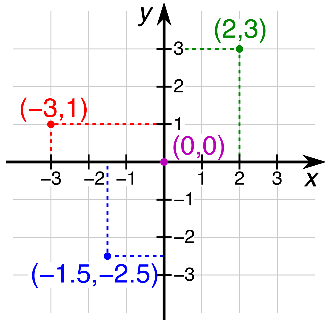
Because these are number lines, direction dictates the mathematical sign. Moving to the right of the y-axis corresponds to a positive x-coordinate, while moving to the left of the y-axis corresponds to a negative x-coordinate. Vertically, moving above the x-axis corresponds to a positive y-coordinate, and moving below the x-axis corresponds to a negative y-coordinate.
The intersection of the infinitely long x-axis and y-axis divides the coordinate plane into four distinct, infinite regions called quadrants. By mathematical convention, these quadrants are traditionally numbered counterclockwise starting from the top right quadrant.
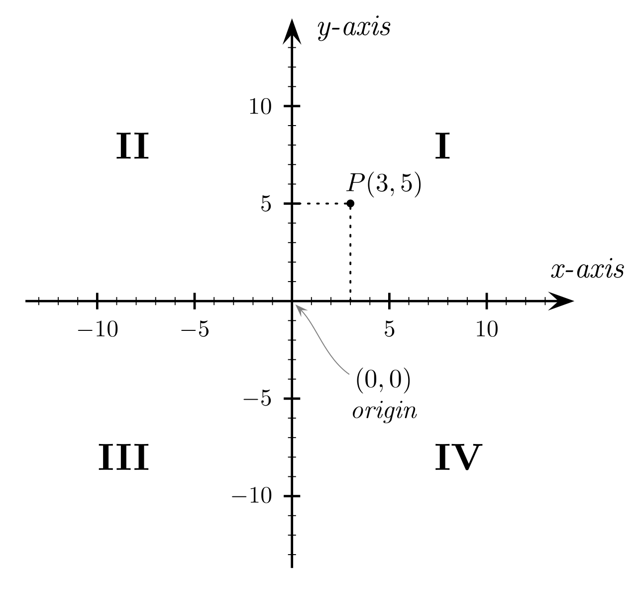
Understanding the behavior of signs in each quadrant allows you to instantly visualize a point's location just by looking at its ordered pair:
| Quadrant | Location | Sign Configuration | Description |
|---|---|---|---|
| Quadrant I | Top Right | (+,+) | Contains points with a positive x-coordinate and a positive y-coordinate. |
| Quadrant II | Top Left | (−,+) | Contains points with a negative x-coordinate and a positive y-coordinate. |
| Quadrant III | Bottom Left | (−,−) | Contains points with a negative x-coordinate and a negative y-coordinate. |
| Quadrant IV | Bottom Right | (+,−) | Contains points with a positive x-coordinate and a negative y-coordinate. |
Once we can plot single points, we can begin charting relationships between variables. The simplest and most profound relationship is the linear one.
Formally, a linear equation is an algebraic equation in which each term is either a constant or the product of a constant and a single variable to the first power. You will never see an x2, a y, or variables multiplied together like xy in a strictly linear equation. Because the variables change at a perfectly constant rate relative to one another, the graph of a linear equation on a Cartesian coordinate plane is always a straight line.
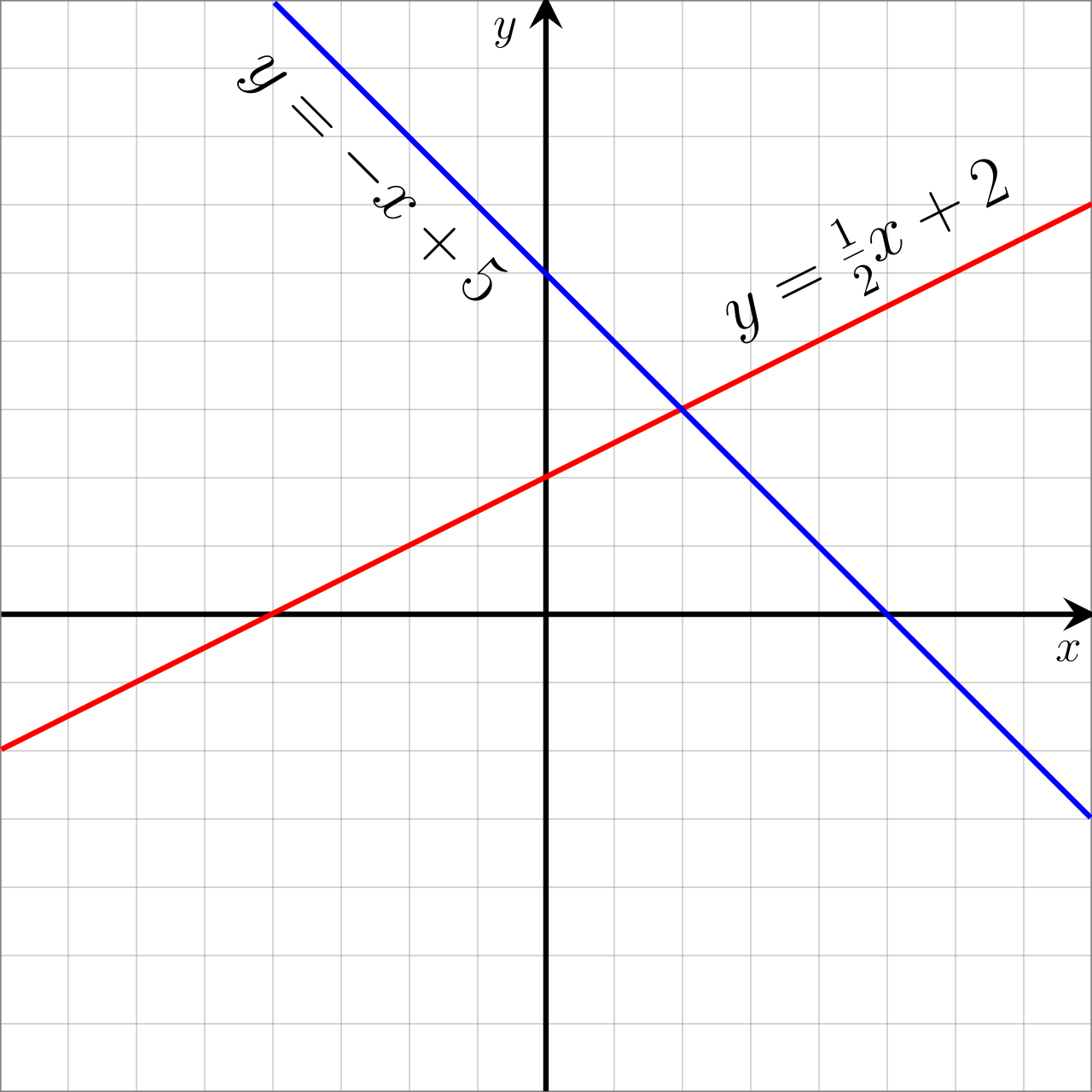
To anchor a line in space, you do not need infinite data. Geometric law dictates that a minimum of two distinct points is required to graph a specific straight line on a coordinate plane. Once you have two points, their trajectory is locked; the line extends infinitely in both directions.
If you are asked to describe a staircase, you might mention how steep it is and whether it is going up or down. In mathematics, we use a single, powerful number to encapsulate both of these properties: the slope.
The slope of a line measures the steepness and the direction of that line. It is calculated as the ratio of the vertical change (the "rise") to the horizontal change (the "run") between any two points on a given line.
The Slope Formula The formula for the slope between two points (x1,y1) and (x2,y2) is: m=x2−x1y2−y1
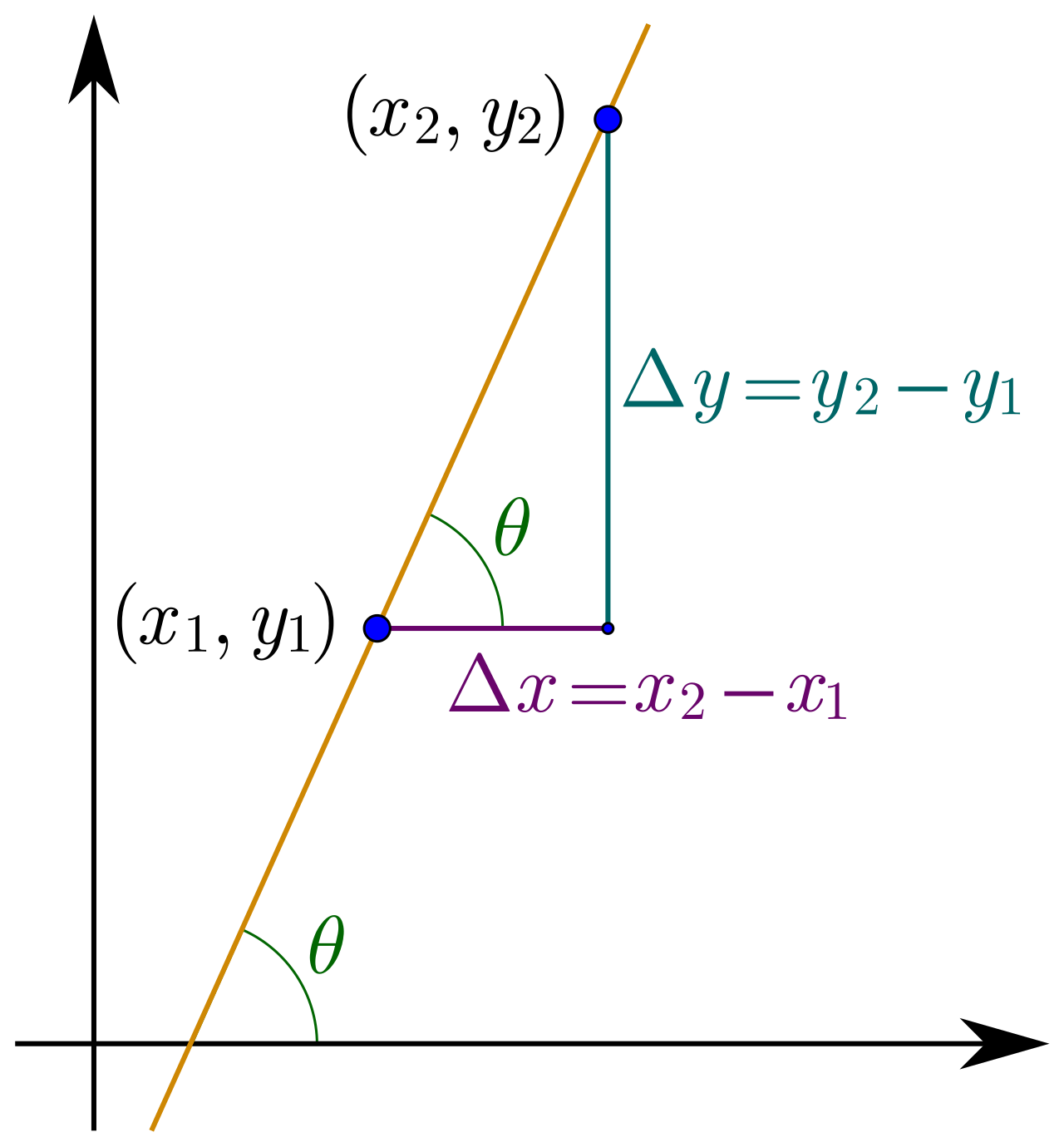
By looking at the calculated slope, we immediately understand the line's visual behavior. There are four distinct realities for slope:
- Positive Slope: A line with a positive slope slants upward from left to right across the coordinate plane. As the x-value increases, the y-value increases.
- Negative Slope: A line with a negative slope slants downward from left to right across the coordinate plane. As the x-value increases, the y-value decreases.
- Zero Slope: A line with a slope of zero forms a perfectly horizontal line on the coordinate plane. There is no vertical "rise" no matter how far you "run". The equation of a horizontal line is written in the form y=c, where c is a constant number representing the fixed y-value.
- Undefined Slope: Consider what happens when you have a perfectly vertical line. The horizontal change—the "run"—between any two points on that line is zero. Because division by zero is undefined in mathematics, the slope of any perfectly vertical line is mathematically undefined. The equation of a vertical line is written in the form x=c, where c is a constant number.
Lines stretch to infinity, but they are most easily understood by where they cross our fundamental axes. These crossing points are called intercepts.
- The x-intercept of a line is the exact point where the line crosses the x-axis. Because the point rests exactly on the horizontal axis, it has not moved up or down. Therefore, the y-coordinate of any x-intercept point is always exactly zero.
- The y-intercept of a line is the exact point where the line crosses the y-axis. Because the point rests exactly on the vertical axis, it has not moved left or right. Therefore, the x-coordinate of any y-intercept point is always exactly zero.
Mathematicians write linear equations in three primary formats, each engineered to reveal different architectural features of the line at a glance.
1. Slope-Intercept Form
The most common and intuitively visual equation of a line.
y=mx+b
In the slope-intercept equation y=mx+b, the variable m represents the slope of the line, dictating its angle. The variable b represents the y-intercept of the line, dictating where the line drops anchor on the vertical axis.
(Note: Because vertical lines have an undefined slope, the graph of a vertical line cannot be written in the slope-intercept form y=mx+b. It requires the separate format x=c.)
2. Standard Form
Often used when solving systems of equations, this form gathers the variables on one side of the equation.
Ax+By=C
The standard form of a linear equation is represented by the formula Ax+By=C, where A, B, and C are generally integers, and A and B are not both zero.
3. Point-Slope Form
This form is the raw algebraic translation of the slope formula itself, incredibly useful when you are given a random point on the line and the slope, but you do not explicitly know the y-intercept.
y−y1=m(x−x1)
The point-slope form of a linear equation is represented by this formula, where (x1,y1) is a known point on the line and m is the slope.
Understanding the properties of a line allows us to reverse-engineer its graph from its equation. Because we know a minimum of two distinct points is required to graph a specific straight line, our goal when graphing is simply to find two reliable, accurate points. There are two highly efficient methods to do this.
Method 1: Graphing via Intercepts If an equation is presented in Standard Form (Ax+By=C), finding the intercepts is extraordinarily fast.
- Set y=0 to calculate the x-intercept.
- Set x=0 to calculate the y-intercept.
- To plot a line using the x-intercept and y-intercept, simply graph the two intercept points on the respective axes and draw a straight line through them.
Method 2: Graphing via Slope-Intercept If an equation is presented in Slope-Intercept form (y=mx+b), the instructions for drawing the line are practically spelled out in the equation.
- Identify the y-intercept (b).
- To plot a line from slope-intercept form, start by graphing the y-intercept point on the y-axis.
- From that anchor point, apply the slope ratio (m, or "rise over run") to traverse to and plot a second point.
- Draw a straight line extending continuously through both points.
By breaking down the coordinate plane into its fundamental components—axes, quadrants, slopes, and intercepts—you move beyond rote memorization. You achieve a structural, visual fluency with algebra.